众所周知,Transformer已经席卷深度学习领域。Transformer架构最初在NLP领域取得了突破性成果,尤其是在机器翻译和语言模型中,其自注意力机制允许模型处理序列数据的全局依赖性。随之,研究者开始探索如何将这种架构应用于计算机视觉任务,特别是目标检测,这是计算机视觉中的核心问题之一。

在目标识别方面,Facebook提出的DETR(Detection Transformer)是第一个将Transformer的核心思想引入到目标检测的模型,它抛弃了传统检测框架中的锚框和区域提案步骤,实现了端到端的检测。
本文将使用四个预训练的DETR模型(DETR ResNet50、DETR ResNet50 DC5、DETR ResNet101和DETR ResNet101 DC5)在自定义数据集上对其进行微调,通过比较它们在自定义数据集上的mAP,来比较评估每个模型的检测精度。
DETR模型结构
如图所示,DETR模型通过将卷积神经网络CNN与Transformer架构相结合,来确定最终的一组边界框。

在目标检测中,预测的Bounding box经过非极大值抑制NMS处理,获得最终的预测。但是,DETR默认总是预测100个Bounding box(可以配置)。因此,我们需要一种方法将真实Bounding box与预测的Bounding box进行匹配。为此,DETR使用了二分图匹配法。
DETR的架构如下图所示。
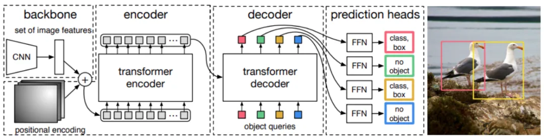
DETR使用CNN模型作为Backbone,在官方代码中,选用的是ResNet架构。CNN学习二维表示,并将输出展平,再进入位置编码(positional encoding)阶段。位置编码后的特征进入Transformer编码器,编码器学习位置嵌入(positional embeddings)。这些位置嵌入随后传递给解码器。解码器的输出嵌入会进一步传递给前馈网络(FFN)。FFN负责识别是物体类别的边界框还是'no object'类别。它会对每个解码器输出进行分类,以确定是否检测到对象以及对应的类别。
DETR模型的详细架构如下:

数据集
本文将使用一个包含多种海洋生物的水族馆数据集(https://www.kaggle.com/datasets/sovitrath/aquarium-data)训练DETR模型。数据集目录结构如下:
Aquarium Combined.v2-raw-1024.voc
├── test [126 entries exceeds filelimit, not opening dir]
├── train [894 entries exceeds filelimit, not opening dir]
├── valid [254 entries exceeds filelimit, not opening dir]
├── README.dataset.txt
└── README.roboflow.txt
其中,数据集包含三个子目录,分别存储图像和注释。注释是以XML(Pascal VOC)格式提供的。训练目录包含了894个图像和注释的组合,训练集447张图像。同理,测试集63张图像,验证集127张图像。
数据集中共有7个类别:
- fish
- jellyfish
- penguin
- shark
- puffin
- stingray
- starfish
准备vision_transformers库
vision_transformers库是一个专注于基于Transformer的视觉模型的新库。尽管Facebook提供了DETR模型的官方仓库,但使用它来进行模型的微调可能较为复杂。vision_transformers库中包含了预训练模型,支持图像分类和对象检测。在这篇文章中,我们将主要关注目标检测模型,库中已经集成了四种DETR模型。
首先,在终端或命令行中使用以下命令克隆vision_transformers库。克隆完成后,使用cd命令进入新克隆的目录。
git clone https://github.com/sovit-123/vision_transformers.git
cd vision_transformers
接下来,我们需要安装PyTorch。最好从官方网站上按照适当的CUDA版本安装PyTorch。例如,以下命令安装了支持CUDA 11.7的PyTorch 2.0.0:
conda install pytorch torchvision torchaudio pytorch-cuda=11.7 -c pytorch -c nvidia安装其它依赖库。
pip install -r requirements.txt在克隆了vision_transformers仓库后,可以再执行以下命令获取库中的所有训练和推理代码。
pip install vision_transformers搭建DETR训练目录
在开始训练DETR模型之前,需要创建一个项目目录结构,以组织代码、数据、日志和模型检查点。
├── input
│   ├── Aquarium Combined.v2-raw-1024.voc
│   └── inference_data
└── vision_transformers
    ├── data
    ├── examples
    ├── example_test_data
    ├── readme_images
    ├── runs
    ├── tools
    ├── vision_transformers
    ├── README.md
    ├── requirements.txt
    └── setup.py
其中:
- input目录:包含水族馆数据集,inference_data目录存放后续用于推理的图像或视频文件。
- vision_transformers目录:这是前面克隆的库。
- tools目录:包含训练和推理所需的脚本,例如train_detector.py(用于训练检测器的脚本)、inference_image_detect.py(用于图像推理的脚本)和inference_video_detect.py(用于视频推理的脚本)
- data目录:包含一些YAML文件,用于模型训练。
训练DETR模型
由于要在自定义数据集上训练4种不同的检测变换器模型,如若对每个模型训练相同的轮数,再挑选最佳模型可能会浪费计算资源。
这里首先对每个模型进行20个训练周期。然后,对在初步训练中表现最佳的模型进行更多轮的训练,以进一步提升模型的性能。
开始训练之前,需要先创建数据集的YAML配置文件。
1.创建数据集YAML配置文件
数据集的YAML文件将存储在vision_transformers/data目录下。它包含了数据集的所有信息。包括图像路径、注释路径、所有类别名称、类别数量等。
vision_transformers库中已经包含了水族馆数据集的YAML文件,但是需要根据当前目录结构修改,
将以下数据复制并粘贴到 data/aquarium.yaml 文件中。
# 图像和标签目录相对于train.py脚本的相对路径
TRAIN_DIR_IMAGES: '../input/Aquarium Combined.v2-raw-1024.voc/train'
TRAIN_DIR_LABELS: '../input/Aquarium Combined.v2-raw-1024.voc/train'
VALID_DIR_IMAGES: '../input/Aquarium Combined.v2-raw-1024.voc/valid'
VALID_DIR_LABELS: '../input/Aquarium Combined.v2-raw-1024.voc/valid'
# 类名
CLASSES: [
    '__background__',
    'fish', 'jellyfish', 'penguin',
    'shark', 'puffin', 'stingray',
    'starfish'
]
# 类别数
NC: 8
# 是否在训练期间保存验证集的预测结果
SAVE_VALID_PREDICTION_IMAGES: True
2.训练模型
训练环境:
- 10GB RTX 3080 GPU
- 10代i7 CPU
- 32GB RAM
(1) 训练DETR ResNet50
执行以下命令:
python tools/train_detector.py --epochs 20 --batch 2 --data data/aquarium.yaml --model detr_resnet50 --name detr_resnet50其中:
- --epochs:模型训练的轮数。
- --batch:数据加载器的批次大小。
- --data:指向数据集YAML文件的路径。
- --model:模型名称。
- --name:保存所有训练结果的目录名,包括训练好的权重。
通过在验证集上计算mAP(Mean Average Precision)来评估目标检测性能。
以下是最佳epoch的检测性能结果。
IoU metric: bbox
 Average Precision  (AP) @[ IoU=0.50:0.95 | area=   all | maxDets=100 ] = 0.172
 Average Precision  (AP) @[ IoU=0.50      | area=   all | maxDets=100 ] = 0.383
 Average Precision  (AP) @[ IoU=0.75      | area=   all | maxDets=100 ] = 0.126
 Average Precision  (AP) @[ IoU=0.50:0.95 | area= small | maxDets=100 ] = 0.094
 Average Precision  (AP) @[ IoU=0.50:0.95 | area=medium | maxDets=100 ] = 0.107
 Average Precision  (AP) @[ IoU=0.50:0.95 | area= large | maxDets=100 ] = 0.247
 Average Recall     (AR) @[ IoU=0.50:0.95 | area=   all | maxDets=  1 ] = 0.088
 Average Recall     (AR) @[ IoU=0.50:0.95 | area=   all | maxDets= 10 ] = 0.250
 Average Recall     (AR) @[ IoU=0.50:0.95 | area=   all | maxDets=100 ] = 0.337
 Average Recall     (AR) @[ IoU=0.50:0.95 | area= small | maxDets=100 ] = 0.235
 Average Recall     (AR) @[ IoU=0.50:0.95 | area=medium | maxDets=100 ] = 0.330
 Average Recall     (AR) @[ IoU=0.50:0.95 | area= large | maxDets=100 ] = 0.344
BEST VALIDATION mAP: 0.17192136022687962
SAVING BEST MODEL FOR EPOCH: 20
由此可以看到模型在不同IoU阈值和目标尺寸条件的表现。
模型在最后一个epoch,IoU阈值0.50到0.95之间对目标检测的平均精度mAP达到了17.2%。
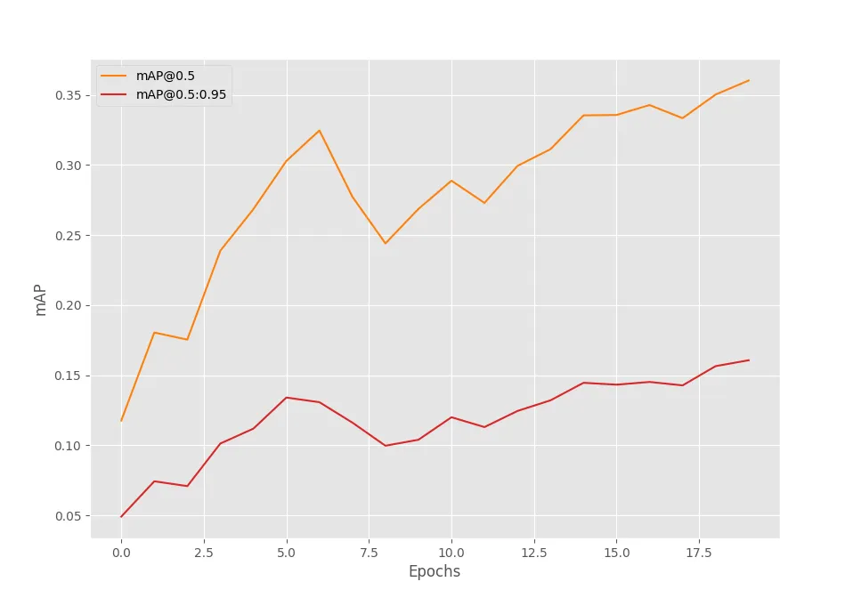
在水族馆数据集上训练DETR ResNet50模型20个epoch后的mAP结果如下图所示。
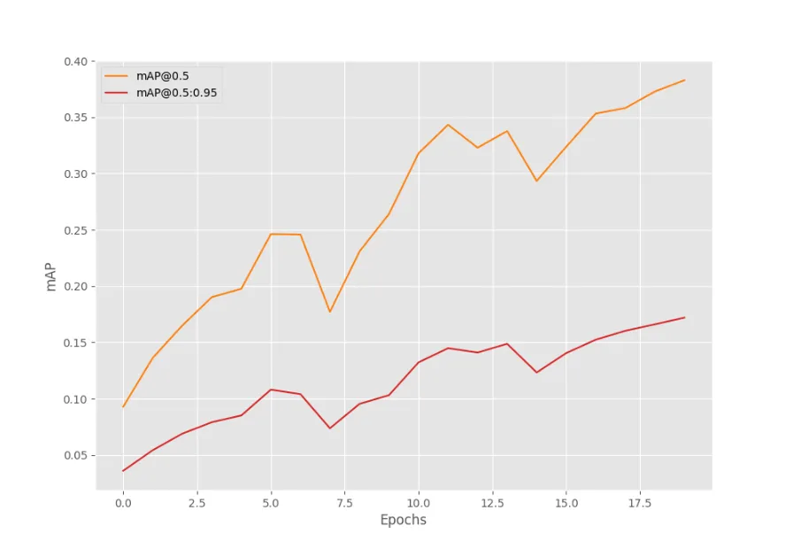
显然,mAP值在逐步提高。但在得出任何结论之前,我们需要对其他模型进行训练。
(2) 训练DETR ResNet50 DC5
执行以下命令:
python tools/train_detector.py --epochs 20 --batch 2 --data data/aquarium.yaml --model detr_resnet50_dc5 --name detr_resnet50_dc5最佳epoch的检测性能结果如下。
Average Precision (AP) @[ IoU=0.50:0.95 | area= all | maxDets=100 ] = 0.161
Average Precision (AP) @[ IoU=0.50 | area= all | maxDets=100 ] = 0.360
Average Precision (AP) @[ IoU=0.75 | area= all | maxDets=100 ] = 0.123
Average Precision (AP) @[ IoU=0.50:0.95 | area= small | maxDets=100 ] = 0.141
Average Precision (AP) @[ IoU=0.50:0.95 | area=medium | maxDets=100 ] = 0.155
Average Precision (AP) @[ IoU=0.50:0.95 | area= large | maxDets=100 ] = 0.233
Average Recall (AR) @[ IoU=0.50:0.95 | area= all | maxDets= 1 ] = 0.096
Average Recall (AR) @[ IoU=0.50:0.95 | area= all | maxDets= 10 ] = 0.248
Average Recall (AR) @[ IoU=0.50:0.95 | area= all | maxDets=100 ] = 0.345
Average Recall (AR) @[ IoU=0.50:0.95 | area= small | maxDets=100 ] = 0.379
Average Recall (AR) @[ IoU=0.50:0.95 | area=medium | maxDets=100 ] = 0.373
Average Recall (AR) @[ IoU=0.50:0.95 | area= large | maxDets=100 ] = 0.340
BEST VALIDATION mAP: 0.16066837142161672
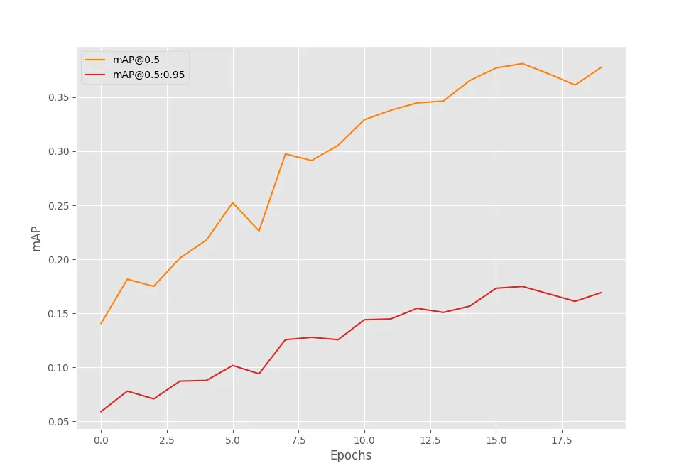
SAVING BEST MODEL FOR EPOCH: 20DETR ResNet50 DC5模型在第20个epoch也达到了最高mAP值,为0.16%,相比于DETR ResNet50模型,这个值较低。
(3) 训练DETR ResNet101
DETR ResNet101模型拥有超过6000万个参数,相较于前两个模型(DETR ResNet50及其DC5变体),网络容量更大。理论上,理论上能够学习到更复杂的特征表示,从而在性能上有所提升。
python tools/train_detector.py --epochs 20 --batch 2 --data data/aquarium.yaml --model detr_resnet101 --name detr_resnet101Average Precision (AP) @[ IoU=0.50:0.95 | area= all | maxDets=100 ] = 0.175
Average Precision (AP) @[ IoU=0.50 | area= all | maxDets=100 ] = 0.381
Average Precision (AP) @[ IoU=0.75 | area= all | maxDets=100 ] = 0.132
Average Precision (AP) @[ IoU=0.50:0.95 | area= small | maxDets=100 ] = 0.089
Average Precision (AP) @[ IoU=0.50:0.95 | area=medium | maxDets=100 ] = 0.113
Average Precision (AP) @[ IoU=0.50:0.95 | area= large | maxDets=100 ] = 0.260
Average Recall (AR) @[ IoU=0.50:0.95 | area= all | maxDets= 1 ] = 0.095
Average Recall (AR) @[ IoU=0.50:0.95 | area= all | maxDets= 10 ] = 0.269
Average Recall (AR) @[ IoU=0.50:0.95 | area= all | maxDets=100 ] = 0.362
Average Recall (AR) @[ IoU=0.50:0.95 | area= small | maxDets=100 ] = 0.298
Average Recall (AR) @[ IoU=0.50:0.95 | area=medium | maxDets=100 ] = 0.451
Average Recall (AR) @[ IoU=0.50:0.95 | area= large | maxDets=100 ] = 0.351
BEST VALIDATION mAP: 0.17489964894400944
SAVING BEST MODEL FOR EPOCH: 17DETR ResNet101模型在第17个epoch达到了17.5%的mAP,相比之前的DETR ResNet50和DETR ResNet50 DC5模型稍有提升,但提升幅度不大。
(4) 训练DETR ResNet101 DC5
DETR ResNet101 DC5模型设计上特别考虑了对小物体检测的优化。本文所用数据集中包含大量小尺寸对象,理论上,DETR ResNet101 DC5模型应该能展现出优于前几个模型的性能。
python tools/train_detector.py --epochs 20 --batch 2 --data data/aquarium.yaml --model detr_resnet101_dc5 --name detr_resnet101_dc5IoU metric: bbox
Average Precision (AP) @[ IoU=0.50:0.95 | area= all | maxDets=100 ] = 0.206
Average Precision (AP) @[ IoU=0.50 | area= all | maxDets=100 ] = 0.438
Average Precision (AP) @[ IoU=0.75 | area= all | maxDets=100 ] = 0.178
Average Precision (AP) @[ IoU=0.50:0.95 | area= small | maxDets=100 ] = 0.110
Average Precision (AP) @[ IoU=0.50:0.95 | area=medium | maxDets=100 ] = 0.093
Average Precision (AP) @[ IoU=0.50:0.95 | area= large | maxDets=100 ] = 0.303
Average Recall (AR) @[ IoU=0.50:0.95 | area= all | maxDets= 1 ] = 0.099
Average Recall (AR) @[ IoU=0.50:0.95 | area= all | maxDets= 10 ] = 0.287
Average Recall (AR) @[ IoU=0.50:0.95 | area= all | maxDets=100 ] = 0.391
Average Recall (AR) @[ IoU=0.50:0.95 | area= small | maxDets=100 ] = 0.317
Average Recall (AR) @[ IoU=0.50:0.95 | area=medium | maxDets=100 ] = 0.394
Average Recall (AR) @[ IoU=0.50:0.95 | area= large | maxDets=100 ] = 0.394
BEST VALIDATION mAP: 0.20588343074278573
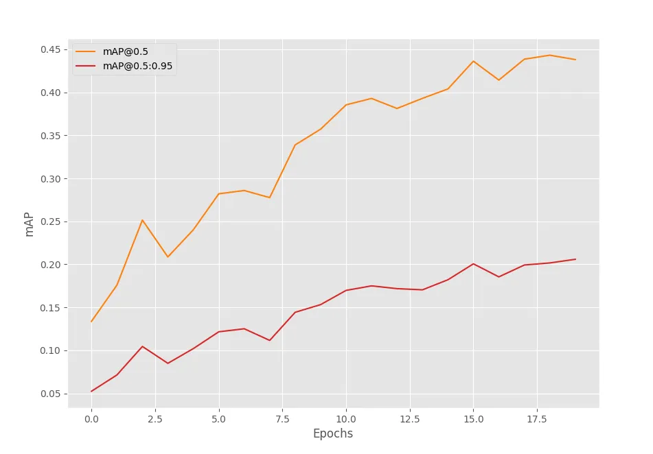
SAVING BEST MODEL FOR EPOCH: 20DETR ResNet101 DC5模型在第20个epoch达到了20%的mAP,这是目前为止的最佳表现。这证实了我们的预期——由于该模型在设计上对小尺寸目标检测进行了优化,因此在含有大量小对象的数据集上,它的性能确实更胜一筹。
接下来,延长训练至60个epochs。由如下结果可以看出,DETR ResNet101 DC5模型在第48个epoch达到了最佳性能,这表明模型在这个阶段找到了更优的权重组合。
 Average Precision  (AP) @[ IoU=0.50:0.95 | area=   all | maxDets=100 ] = 0.239
 Average Precision  (AP) @[ IoU=0.50      | area=   all | maxDets=100 ] = 0.501
 Average Precision  (AP) @[ IoU=0.75      | area=   all | maxDets=100 ] = 0.186
 Average Precision  (AP) @[ IoU=0.50:0.95 | area= small | maxDets=100 ] = 0.119
 Average Precision  (AP) @[ IoU=0.50:0.95 | area=medium | maxDets=100 ] = 0.143
 Average Precision  (AP) @[ IoU=0.50:0.95 | area= large | maxDets=100 ] = 0.328
 Average Recall     (AR) @[ IoU=0.50:0.95 | area=   all | maxDets=  1 ] = 0.109
 Average Recall     (AR) @[ IoU=0.50:0.95 | area=   all | maxDets= 10 ] = 0.290
 Average Recall     (AR) @[ IoU=0.50:0.95 | area=   all | maxDets=100 ] = 0.394
 Average Recall     (AR) @[ IoU=0.50:0.95 | area= small | maxDets=100 ] = 0.349
 Average Recall     (AR) @[ IoU=0.50:0.95 | area=medium | maxDets=100 ] = 0.369
 Average Recall     (AR) @[ IoU=0.50:0.95 | area= large | maxDets=100 ] = 0.398
BEST VALIDATION mAP: 0.23894132553612263
SAVING BEST MODEL FOR EPOCH: 48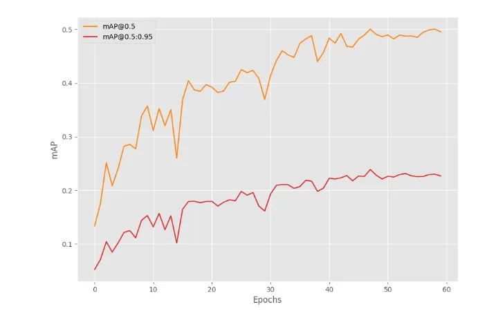
DETR ResNet101 DC5模型在447个训练样本上达到了24%的mAP,对于IoU=0.50:0.95,这样的结果相当不错。
3.推理
(1) 视频推理
使用inference_video_detect.py脚本进行视频推理。将视频文件路径作为输入,脚本就会处理视频中的每一帧,并在每个帧上运行目标检测。
python tools/inference_video_detect.py --weights runs/training/detr_resnet101_dc5_60e/best_model.pth --input ../input/inference_data/video_1.mp4 --show这里多了一个--show标志,它允许在推理过程中实时显示结果,在RTX 3080 GPU上,模型平均可以达到38 FPS的速度。
「inference_video_detect.py」
import torch
import cv2
import numpy as np
import argparse
import yaml
import os
import time
import torchinfo

from vision_transformers.detection.detr.model import DETRModel
from utils.detection.detr.general import (
    set_infer_dir,
    load_weights
)
from utils.detection.detr.transforms import infer_transforms, resize
from utils.detection.detr.annotations import (
    convert_detections,
    inference_annotations,
    annotate_fps,
    convert_pre_track,
    convert_post_track
)
from deep_sort_realtime.deepsort_tracker import DeepSort
from utils.detection.detr.viz_attention import visualize_attention

# NumPy随机数生成器的种子值为2023
np.random.seed(2023)

# 命令行参数配置选项
def parse_opt():
    parser = argparse.ArgumentParser()
    # 模型权重文件的路径
    parser.add_argument(
        '-w',
        '--weights',
    )
    # 输入图像或图像文件夹的路径
    parser.add_argument(
        '-i', '--input',
        help='folder path to input input image (one image or a folder path)',
    )
    # 数据配置文件的路径
    parser.add_argument(
        '--data',
        default=None,
        help='(optional) path to the data config file'
    )
    # 模型名称,默认为'detr_resnet50'
    parser.add_argument(
        '--model',
        default='detr_resnet50',
        help='name of the model'
    )
    # 计算和训练设备,默认使用GPU(如果可用)否则使用CPU
    parser.add_argument(
        '--device',
        default=torch.device('cuda:0' if torch.cuda.is_available() else 'cpu'),
        help='computation/training device, default is GPU if GPU present'
    )
    # 图像的尺寸,默认为640
    parser.add_argument(
        '--imgsz',
        '--img-size',
        default=640,
        dest='imgsz',
        type=int,
        help='resize image to, by default use the original frame/image size'
    )
    # 可视化时的置信度阈值,默认为0.5
    parser.add_argument(
        '-t',
        '--threshold',
        type=float,
        default=0.5,
        help='confidence threshold for visualization'
    )
    # 训练结果存放目录
    parser.add_argument(
        '--name',
        default=None,
        type=str,
        help='training result dir name in outputs/training/, (default res_#)'
    )
    # 不显示边界框上的标签
    parser.add_argument(
        '--hide-labels',
        dest='hide_labels',
        action='store_true',
        help='do not show labels during on top of bounding boxes'
    )
    # 只有传递该选项时才会显示输出
    parser.add_argument(
        '--show',
        dest='show',
        action='store_true',
        help='visualize output only if this argument is passed'
    )
    # 开启跟踪功能
    parser.add_argument(
        '--track',
        action='store_true'
    )
    # 过滤要可视化的类别,如--classes 1 2 3
    parser.add_argument(
        '--classes',
        nargs='+',
        type=int,
        default=None,
        help='filter classes by visualization, --classes 1 2 3'
    )
    # 可视化检测框的注意力图
    parser.add_argument(
        '--viz-atten',
        dest='vis_atten',
        action='store_true',
        help='visualize attention map of detected boxes'
    )
    args = parser.parse_args()
    return args

# 读取并处理视频文件相关信息
def read_return_video_data(video_path):
    # 打开指定路径的视频文件
    cap = cv2.VideoCapture(video_path)
    # 获取视频帧的宽度和高度
    frame_width = int(cap.get(3))
    frame_height = int(cap.get(4))
    # 获取视频的帧率
    fps = int(cap.get(5))
    # 检查视频的宽度和高度是否不为零。如果它们都是零,那么会抛出一个错误消息,提示用户检查视频路径是否正确
    assert (frame_width != 0 and frame_height !=0), 'Please check video path...'
    # 函数返回一个元组,包含VideoCapture对象cap以及视频的宽度、高度和帧率fps
    return cap, frame_width, frame_height, fps

def main(args):
    # 如果args.track为真,初始化DeepSORT追踪器
    if args.track:
        tracker = DeepSort(max_age=30)
    # 根据args.data加载数据配置(如果存在)以获取类别数量和类别列表
    NUM_CLASSES = None
    CLASSES = None
    data_configs = None
    if args.data is not None:
        with open(args.data) as file:
            data_configs = yaml.safe_load(file)
        NUM_CLASSES = data_configs['NC']
        CLASSES = data_configs['CLASSES']
    # 获取设备类型
    DEVICE = args.device
    # 设置输出目录
    OUT_DIR = set_infer_dir(args.name)
    # 加载模型权重
    model, CLASSES, data_path = load_weights(
        args,
        # 设备类型
        DEVICE,
        # 模型类
        DETRModel,
        # 数据配置
        data_configs,
        # 类别数量
        NUM_CLASSES,
        # 类别列表
        CLASSES,
        video=True
    )
    # 将模型移动到指定的设备(如GPU或CPU)并将其设置为评估模式(.eval())
    _ = model.to(DEVICE).eval()
    # 使用torchinfo.summary来打印模型的详细结构和参数统计
    try:
        torchinfo.summary(
            model,
            device=DEVICE,
            input_size=(1, 3, args.imgsz, args.imgsz),
            row_settings=["var_names"]
        )
    # 如果此过程出现异常,代码会打印模型的完整结构,并计算模型的总参数数和可训练参数数
    except:
        print(model)
        # 计算模型的所有参数总数
        total_params = sum(p.numel() for p in model.parameters())
        print(f"{total_params:,} total parameters.")
        # 只计算那些需要在训练过程中更新的参数(即requires_grad属性为True的参数)
        total_trainable_params = sum(
            p.numel() for p in model.parameters() if p.requires_grad)
        print(f"{total_trainable_params:,} training parameters.")

    # 生成一个随机分布的颜色数组,每个元素的值在0到255之间,这是标准的8位RGB色彩空间中的每个通道的取值范围
    COLORS = np.random.uniform(0, 255, size=(len(CLASSES), 3))
    # 获取视频的路径
    VIDEO_PATH = args.input
    # 如果用户没有通过命令行参数--input指定视频路径,则将VIDEO_PATH设置为data_path
    if VIDEO_PATH == None:
        VIDEO_PATH = data_path
    # cap: 一个cv2.VideoCapture对象,用于读取和处理视频文件
    # frame_width: 视频的帧宽度(宽度像素数)
    # frame_height: 视频的帧高度(高度像素数)
    # fps: 视频的帧率(每秒帧数)
    cap, frame_width, frame_height, fps = read_return_video_data(VIDEO_PATH)
    # 生成输出文件的名称
    # [-1]:选取列表中的最后一个元素,即文件名(包括扩展名)
    # .split('.')[0]:再次分割文件名,这次是基于点号(.)来分隔,然后选取第一个元素,即文件的基本名称,不包括扩展名
    save_name = VIDEO_PATH.split(os.path.sep)[-1].split('.')[0]
    # 将处理后的帧写入输出视频文件
    # 输出文件路径:f"{OUT_DIR}/{save_name}.mp4"
    # 编码器(codec):cv2.VideoWriter_fourcc(*'mp4v')
    # 帧率(fps)
    # 视频尺寸:(frame_width, frame_height)
    out = cv2.VideoWriter(f"{OUT_DIR}/{save_name}.mp4",
                        cv2.VideoWriter_fourcc(*'mp4v'), fps,
                        (frame_width, frame_height))
    # 检查args.imgsz是否已设置(即用户是否通过命令行参数指定了图像大小)
    # 如果args.imgsz有值,说明用户想要将输入图像(或视频帧)缩放到指定的大小,那么RESIZE_TO将被设置为这个值
    if args.imgsz != None:
        RESIZE_TO = args.imgsz
    # 如果args.imgsz没有设置或者为None,则默认使用视频帧的原始宽度frame_width作为缩放尺寸
    else:
        RESIZE_TO = frame_width
    # 记录总的帧数
    frame_count = 0
    # 计算最终的帧率
    total_fps = 0

    # 检查视频是否已经结束
    while(cap.isOpened()):
        # 读取下一帧,并返回一个布尔值ret表示是否成功读取
        ret, frame = cap.read()
        if ret:
            # 复制原始帧以保留未处理的版本
            orig_frame = frame.copy()
            # 使用resize函数将帧调整到指定的大小(如果args.imgsz已设置,否则保持原大小)
            frame = resize(frame, RESIZE_TO, square=True)
            image = frame.copy()
            # 将BGR图像转换为RGB
            image = cv2.cvtColor(image, cv2.COLOR_BGR2RGB)
            # 将图像归一化到0-1范围
            image = image / 255.0
            # 预处理
            image = infer_transforms(image)
            # 将图像转换为PyTorch张量,设置数据类型为torch.float32
            image = torch.tensor(image, dtype=torch.float32)
            # 调整张量维度,使通道维度成为第一个维度,以便于模型输入(模型通常期望输入张量的形状为(batch_size, channels, height, width))
            image = torch.permute(image, (2, 0, 1))
            # 在张量前面添加一个维度以表示批次大小(batch_size=1)
            image = image.unsqueeze(0)

            # 计算模型前向传播的时间(start_time和forward_end_time)以衡量处理单帧的速度
            start_time = time.time()
            with torch.no_grad():
                outputs = model(image.to(args.device))
            forward_end_time = time.time()

            forward_pass_time = forward_end_time - start_time

            # 计算当前帧的处理速度
            fps = 1 / (forward_pass_time)
            # Add `fps` to `total_fps`.
            total_fps += fps
            # Increment frame count.
            frame_count += 1
            # 如果启用了注意力可视化(args.vis_atten),则将注意力图保存为图像文件
            if args.vis_atten:
                visualize_attention(
                    model,
                    image,
                    args.threshold,
                    orig_frame,
                    f"{OUT_DIR}/frame_{str(frame_count)}.png",
                    DEVICE
                )
            # 如果模型检测到了物体(outputs['pred_boxes'][0]非空)
            if len(outputs['pred_boxes'][0]) != 0:
                # 转换预测结果
                draw_boxes, pred_classes, scores = convert_detections(
                    outputs,
                    args.threshold,
                    CLASSES,
                    orig_frame,
                    args
                )
                # 使用tracker更新跟踪状态,并将结果转换回检测框(convert_pre_track和convert_post_track)
                if args.track:
                    tracker_inputs = convert_pre_track(
                        draw_boxes, pred_classes, scores
                    )
                    # Update tracker with detections.
                    tracks = tracker.update_tracks(
                        tracker_inputs, frame=frame
                    )
                    draw_boxes, pred_classes, scores = convert_post_track(tracks)
                # 将预测结果应用到原始帧上(inference_annotations),包括绘制边界框、类别标签和置信度
                orig_frame = inference_annotations(
                    draw_boxes,
                    pred_classes,
                    scores,
                    CLASSES,
                    COLORS,
                    orig_frame,
                    args
                )
            # 在帧上添加实时FPS信息
            orig_frame = annotate_fps(orig_frame, fps)
            # 将处理后的帧写入输出视频文件
            out.write(orig_frame)
            if args.show:
                cv2.imshow('Prediction', orig_frame)
                # Press `q` to exit
                if cv2.waitKey(1) & 0xFF == ord('q'):
                    break
        else:
            break
    if args.show:
        # Release VideoCapture().
        cap.release()
        # Close all frames and video windows.
        cv2.destroyAllWindows()

    # Calculate and print the average FPS.
    avg_fps = total_fps / frame_count
    print(f"Average FPS: {avg_fps:.3f}")

if __name__ == '__main__':
    args = parse_opt()
    main(args)
视频1推理结果如下。尽管模型在大部分情况下表现良好,但是误将corals识别为fish了。通过提高阈值,可以减少假阳性,即模型错误识别为fish的corals。
视频2推理结果如下。考虑到模型在未知环境中表现出的性能,这些结果是相当不错的。误将stingrays识别为fish类的情况可能是由于它们在形状和外观上与某些鱼类相似,这导致模型在分类时出现混淆。不过,总体来说,模型的检测效果还是令人满意的。
(2) 图片推理
有了最佳训练权重,现在可以进行推理测试了。
python tools/inference_image_detect.py --weights runs/training/detr_resnet101_dc5_60e/best_model.pth --input "../input/Aquarium Combined.v2-raw-1024.voc/test"其中:
- --weights:表示用于推理的权重文件路径。这里即指训练60个epoch后得到的最佳模型权重的路径。
- --input:推理测试图像所在目录。
「inference_image_detect.py」
import torch
import cv2
import numpy as np
import argparse
import yaml
import glob
import os
import time
import torchinfo

from vision_transformers.detection.detr.model import DETRModel
from utils.detection.detr.general import (
    set_infer_dir,
    load_weights
)
from utils.detection.detr.transforms import infer_transforms, resize
from utils.detection.detr.annotations import (
    convert_detections,
    inference_annotations,
)
from utils.detection.detr.viz_attention import visualize_attention

np.random.seed(2023)

def parse_opt():
    parser = argparse.ArgumentParser()
    parser.add_argument(
        '-w',
        '--weights',
    )
    parser.add_argument(
        '-i', '--input',
        help='folder path to input input image (one image or a folder path)',
    )
    parser.add_argument(
        '--data',
        default=None,
        help='(optional) path to the data config file'
    )
    parser.add_argument(
        '--model',
        default='detr_resnet50',
        help='name of the model'
    )
    parser.add_argument(
        '--device',
        default=torch.device('cuda:0' if torch.cuda.is_available() else 'cpu'),
        help='computation/training device, default is GPU if GPU present'
    )
    parser.add_argument(
        '--imgsz',
        '--img-size',
        default=640,
        dest='imgsz',
        type=int,
        help='resize image to, by default use the original frame/image size'
    )
    parser.add_argument(
        '-t',
        '--threshold',
        type=float,
        default=0.5,
        help='confidence threshold for visualization'
    )
    parser.add_argument(
        '--name',
        default=None,
        type=str,
        help='training result dir name in outputs/training/, (default res_#)'
    )
    parser.add_argument(
        '--hide-labels',
        dest='hide_labels',
        action='store_true',
        help='do not show labels during on top of bounding boxes'
    )
    parser.add_argument(
        '--show',
        dest='show',
        action='store_true',
        help='visualize output only if this argument is passed'
    )
    parser.add_argument(
        '--track',
        action='store_true'
    )
    parser.add_argument(
        '--classes',
        nargs='+',
        type=int,
        default=None,
        help='filter classes by visualization, --classes 1 2 3'
    )
    parser.add_argument(
        '--viz-atten',
        dest='vis_atten',
        action='store_true',
        help='visualize attention map of detected boxes'
    )
    args = parser.parse_args()
    return args

def collect_all_images(dir_test):
    """
    Function to return a list of image paths.
    :param dir_test: Directory containing images or single image path.
    Returns:
        test_images: List containing all image paths.
    """
    test_images = []
    if os.path.isdir(dir_test):
        image_file_types = ['*.jpg', '*.jpeg', '*.png', '*.ppm']
        for file_type in image_file_types:
            test_images.extend(glob.glob(f"{dir_test}/{file_type}"))
    else:
        test_images.append(dir_test)
    return test_images

def main(args):
    NUM_CLASSES = None
    CLASSES = None
    data_configs = None
    if args.data is not None:
        with open(args.data) as file:
            data_configs = yaml.safe_load(file)
        NUM_CLASSES = data_configs['NC']
        CLASSES = data_configs['CLASSES']

    DEVICE = args.device
    OUT_DIR = set_infer_dir(args.name)

    model, CLASSES, data_path = load_weights(
        args, DEVICE, DETRModel, data_configs, NUM_CLASSES, CLASSES
    )
    _ = model.to(DEVICE).eval()
    try:
        torchinfo.summary(
            model,
            device=DEVICE,
            input_size=(1, 3, args.imgsz, args.imgsz),
            row_settings=["var_names"]
        )
    except:
        print(model)
        # Total parameters and trainable parameters.
        total_params = sum(p.numel() for p in model.parameters())
        print(f"{total_params:,} total parameters.")
        total_trainable_params = sum(
            p.numel() for p in model.parameters() if p.requires_grad)
        print(f"{total_trainable_params:,} training parameters.")

    # Colors for visualization.
    COLORS = np.random.uniform(0, 255, size=(len(CLASSES), 3))
    DIR_TEST = args.input
    if DIR_TEST == None:
        DIR_TEST = data_path
    test_images = collect_all_images(DIR_TEST)
    print(f"Test instances: {len(test_images)}")

    # To count the total number of frames iterated through.
    frame_count = 0
    # To keep adding the frames' FPS.
    total_fps = 0
    for image_num in range(len(test_images)):
        image_name = test_images[image_num].split(os.path.sep)[-1].split('.')[0]
        orig_image = cv2.imread(test_images[image_num])
        frame_height, frame_width, _ = orig_image.shape
        if args.imgsz != None:
            RESIZE_TO = args.imgsz
        else:
            RESIZE_TO = frame_width

        image_resized = resize(orig_image, RESIZE_TO, square=True)
        image = cv2.cvtColor(image_resized, cv2.COLOR_BGR2RGB)
        image = image / 255.0
        image = infer_transforms(image)
        input_tensor = torch.tensor(image, dtype=torch.float32)
        input_tensor = torch.permute(input_tensor, (2, 0, 1))
        input_tensor = input_tensor.unsqueeze(0)
        h, w, _ = orig_image.shape

        start_time = time.time()
        with torch.no_grad():
            outputs = model(input_tensor.to(DEVICE))
        end_time = time.time()
        # Get the current fps.
        fps = 1 / (end_time - start_time)
        # Add `fps` to `total_fps`.
        total_fps += fps
        # Increment frame count.
        frame_count += 1

        if args.vis_atten:
            visualize_attention(
                model,
                input_tensor,
                args.threshold,
                orig_image,
                f"{OUT_DIR}/{image_name}.png",
                DEVICE
            )

        if len(outputs['pred_boxes'][0]) != 0:
            draw_boxes, pred_classes, scores = convert_detections(
                outputs,
                args.threshold,
                CLASSES,
                orig_image,
                args
            )
            orig_image = inference_annotations(
                draw_boxes,
                pred_classes,
                scores,
                CLASSES,
                COLORS,
                orig_image,
                args
            )
            if args.show:
                cv2.imshow('Prediction', orig_image)
                cv2.waitKey(1)

        cv2.imwrite(f"{OUT_DIR}/{image_name}.jpg", orig_image)
        print(f"Image {image_num+1} done...")
        print('-'*50)

    print('TEST PREDICTIONS COMPLETE')
    if args.show:
        cv2.destroyAllWindows()
        # Calculate and print the average FPS.
    avg_fps = total_fps / frame_count
    print(f"Average FPS: {avg_fps:.3f}")

if __name__ == '__main__':
    args = parse_opt()
    main(args)
默认情况下,脚本使用0.5的得分阈值,我们也可以使用--threshold标志来修改这个值。
python tools/inference_image_detect.py \
    --weights /path/to/best/weights.pth \
    --input /path/to/test/images/directory \
    --threshold 0.5
运行这个命令后,脚本会加载模型权重,处理测试图像,并将结果保存在指定的输出目录中,查看生成的图像或结果文件,以评估模型在实际测试集上的表现。
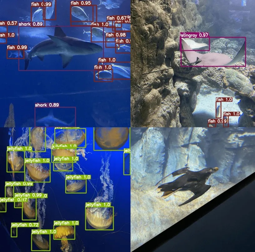
从目前的结果来看,模型在检测sharks、fish和stingrays方面表现得较为高效,但对puffins的检测效果不佳。这很可能是因为训练数据集中这些类别的实例数量较少,导致模型在学习这些特定类别特征时不够充分。