使用 LGBM 等模型预测信用卡潜在客户-51CTO.COM

关于数据集

有一家名为Happy Customer Bank (快乐客户银行) 的银行，是一家中型私人银行，经营各类银行产品，如储蓄账户、往来账户、投资产品、信贷产品等。

该银行还向现有客户交叉销售产品，为此他们使用不同类型的通信方式，如电话、电子邮件、网上银行推荐、手机银行等。

在这种情况下，Happy Customer Bank 希望向现有客户交叉销售其信用卡。该银行已经确定了一组有资格使用这些信用卡的客户。

银行希望确定对推荐的信用卡表现出更高意向的客户。

该数据集主要包括：

客户详细信息（gender, age, region, etc）
他/她与银行的关系详情（Channel_Code、Vintage、Avg_Asset_Value, etc）

在这里，我们的任务是构建一个能够识别对信用卡感兴趣的客户的模型。

导入库

导入必要的库，例如用于线性代数的 NumPy、用于数据处理的 Pandas、Seaborn 和用于数据可视化的 Matplotlib。

import numpy as np  
import pandas as pd  
import matplotlib.pyplot as plt
import seaborn as sns1.
2.
3.
4.

加载数据集

df_train=pd.read_csv("dataset/train_s3TEQDk.csv")
df_train["source"]="train"
df_test=pd.read_csv("dataset/test_mSzZ8RL.csv")
df_test["source"]="test"
df=pd.concat([df_train,df_test],
             ignore_index=True)
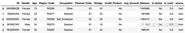
df.head()1.
2.
3.
4.
5.
6.
7.

检查和清洗数据集

加载数据集后，下一步是检查有关数据集的信息并清理数据集，包括检查形状、数据类型、唯一值、缺失值和异常值等。

检查形状

df.shape1.

在我们的数据集中，合并训练和测试文件后，我们有 351037 行，具有 12 个特征。

检查唯一值

df.nunique()
ID                     351037
Gender                      2
Age                        63
Region_Code                35
Occupation                  4
Channel_Code                4
Vintage                    66
Credit_Product              2
Avg_Account_Balance    162137
Is_Active                   2
Is_Lead                     2
source                      2
dtype: int641.
2.
3.
4.
5.
6.
7.
8.
9.
10.
11.
12.
13.
14.

检查缺失值

df.isnull().sum()
ID                          0
Gender                      0
Age                         0
Region_Code                 0
Occupation                  0
Channel_Code                0
Vintage                     0
Credit_Product          41847
Avg_Account_Balance         0
Is_Active                   0
Is_Lead                105312
source                      01.
2.
3.
4.
5.
6.
7.
8.
9.
10.
11.
12.
13.

Credit_Product 特征中存在不少空值。

现在我们使用 fillna 方法来填充数据集中的空值。

#填充空值
df['Credit_Product']= df['Credit_Product'].fillna("NA")1.
2.

我们删除了数据集中存在的所有空值。

检查数据类型

接下来我们必须检查特征的数据类型。

df.info()
<class 'pandas.core.frame.DataFrame'>
RangeIndex: 351037 entries, 0 to 351036
Data columns (total 12 columns):  
#   Column               Non-Null Count   Dtype
---  ------               --------------   -----  
 ID                   351037 non-null  object  
 Gender               351037 non-null  object  
 Age                  351037 non-null  int64    
 Region_Code          351037 non-null  object  
 Occupation           351037 non-null  object  
 Channel_Code         351037 non-null  object  
 Vintage              351037 non-null  int64    
 Credit_Product       351037 non-null  object  
 Avg_Account_Balance  351037 non-null  int64    
 Is_Active            351037 non-null  object  
Is_Lead              245725 non-null  float64  
source               351037 non-null  object  
dtypes: float64(1), int64(3), object(8)
memory usage: 32.1+ MB1.




















观察得到：

一些分类特征需要在数值数据类型中进行更改。
在这里，我们发现 Is_Active 特征有两个值，即 Yes 和 No。因此，我们必须将这些值转换为 float 数据类型。

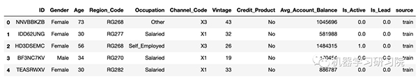
将 Is_Active 列中的 Yes 更改为 1 并将 No 更改为 0 以将数据转换为浮点数。

df["Is_Active"].replace(["Yes","No"]
           ,[1,0], inplace=True)
df['Is_Active'] = df['Is_Active'].astype(float)
df.head()1.
2.
3.
4.

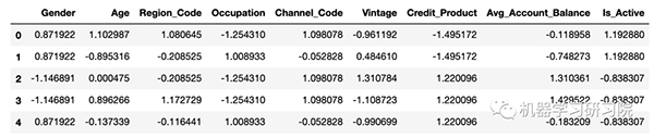
现在，为了将所有分类列更改为数字形式，我们使用标签编码。我们先简要了解标签编码到底是什么。

标签编码：标签编码是指将标签转换为数字形式，以便将其转换为机器可读形式。它是一种用于处理分类变量的流行编码技术。

接下来使用标签编码器。

#创建分类列列表
cat_col=['Gender', 'Region_Code',
       'Occupation','Channel_Code',
       'Credit_Product']
from sklearn.preprocessing import LabelEncoder
le = LabelEncoder()
for col in cat_col:  
   df[col]= le.fit_transform(df[col])

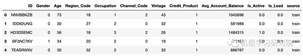
df_2= df
df_2.head()1.
2.
3.
4.
5.
6.
7.
8.
9.
10.
11.

此时，我们可以删除不相关且对我们的数据集没有影响的特征。这里我们有两列要删除，即"ID"和"source"。让我们检查一下最新的输出。

至此，我们观察到所有数据都是数字。

数据可视化

为了更加清晰地分析数据集，数据可视化是一个不可或缺的步骤。

单变量分析

首先，我们绘制了 dist计数图以了解数据的分布。

年龄特征分布密度图

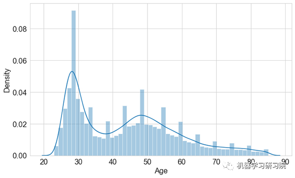
观察得到：

在年龄分布略偏向左侧，即“正偏态”。
在这里，我们看到一个峰值年龄组在 20 到 40 岁之间，该年龄段更加年轻，而另一个峰值年龄组在 40 到 60 岁之间。除此之外，40 到 60 岁之间的人更有优势。
因此，这可能与"Vintage"变量相关联，该变量对于较高年龄组更明显。

性别特征的计数图

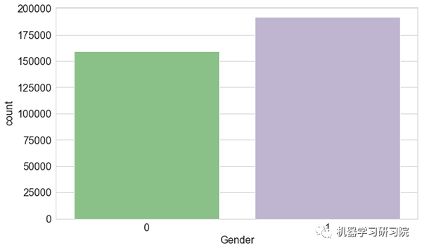
观察得到：

数据集中存在更多男性客户。但是，在决定谁拥有更好的决策权时，客户的性别并不重要。

目标变量计数图

本案例中的目标变量为 Is_Lead 特征。

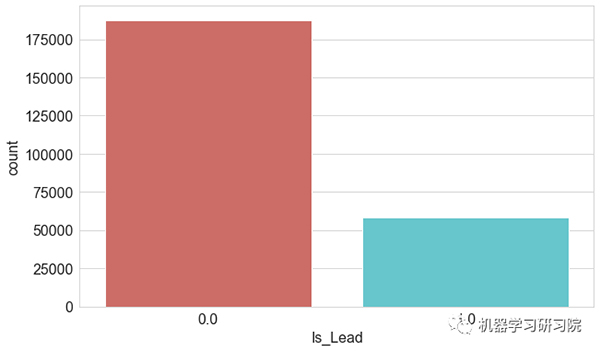
观察得到：

该图显示数据高度不平衡，在应用不同算法之前进行需要对数据集进行平衡处理。
为了平衡数据集，下面的步骤中将会使用欠采样技术。

此处可以参考：机器学习中样本不平衡，怎么办？

双变量分析

接下来做一些双变量分析，以理解不同列之间的关系。

"职业"和"客户"

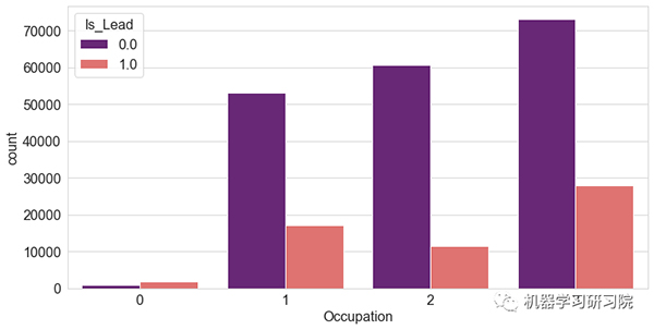
观察得到：

我们观察到自由职业客户不太可能办理信用卡。而企业家（尽管有限）最有可能办理信用卡。

近3个月内不同"客户的职业"的"客户活跃度"

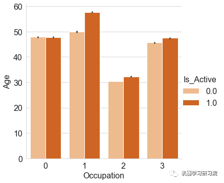
观察得到：

在过去3个月里，与企业家相比，活跃客户更多地来自工薪阶层、个体经营者和其他人群。
与 “活跃” 的客户相比，过去3个月内不活跃的客户相当多。
与 “非活跃” 客户相比，“活跃” 客户的潜在客户比例更高。

数据预处理

正如前所述，该数据集目标变量是不平衡的，需要进行平衡处理以建立有效的建模。

因此我们采用欠采样方法来处理平衡数据集。

接下来首先导入库，再将少数类和多数类分开。

from sklearn.utils import resample
# 将少数类和多数类分开
df_majority = df_1[df_1['Is_Lead']==0]
df_minority = df_1[df_1['Is_Lead']==1]
print("多数类值为", len(df_majority))
print("少数类值是", len(df_minority))
print("两个类的比例是", len(df_majority)/len(df_minority))1.
2.
3.
4.
5.
6.
7.

观察得到：

多数类值为187437，少数类值为58288，两个类的比率为3.2。

现在，需要将少数类与过采样的多数类结合起来。

# 欠采样多数类
df_majority_undersampled = resample(df_majority,
     replace=True,
     n_samples=len(df_minority),
     random_state=0）
# 结合少数类和过采样的多数类
df_undersampled = pd.concat([df_minority,  
         df_majority_undersampled])
df_undersampled['Is_Lead'].value_counts()
df_1=df_undersampled1.
2.
3.
4.
5.
6.
7.
8.
9.
10.

在此之后，我们必须计算新的类值计数。

# 显示新的类值计数
print("欠采样类值计数为：", len(df_undersampled))
print("两个类的比例为：",  
       len(df_undersampled[df_undersampled["Is_Lead"]==0]
       )/len(df_undersampled[df_undersampled["Is_Lead"]==1]))1.
2.
3.
4.
5.

观察得到：

欠采样类值计数为 126800。
两个类的比率为 1.0。

此时需要将特征变量与目标变量分开，并拆分训练集及测试集。

# 删除目标变量  
xc = df_1.drop(columns=['Is_Lead'])
yc = df_1[["Is_Lead"]]1.
2.
3.

现在，我在这里使用 Standard Scaler 对x的值进行标准化以使数据呈正态分布。

sc = StandardScaler()  
#Standard Scaler的实例
df_xc = pd.DataFrame(sc.fit_transform(xc),columns=xc.columns)
df_xc1.
2.
3.
4.

分类模型建立

导入分类建模所需的库

#Importing necessary libraries
from sklearn import metrics
from scipy.stats import zscore
from sklearn.preprocessing import LabelEncoder,StandardScaler
from sklearn.model_selection import train_test_split,GridSearchCV
from sklearn.decomposition import PCA
from sklearn.metrics import precision_score, recall_score, confusion_matrix, f1_score, roc_auc_score, roc_curve
from sklearn.metrics import accuracy_score,classification_report,confusion_matrix,roc_auc_score,roc_curve
from sklearn.metrics import auc
from sklearn.metrics import plot_roc_curve
from sklearn.linear_model import LogisticRegression
from sklearn.naive_bayes import MultinomialNB
from sklearn.neighbors import KNeighborsClassifier
from sklearn.ensemble import RandomForestClassifier
from sklearn.svm import SVC
from sklearn.tree import DecisionTreeClassifier
from sklearn.ensemble import AdaBoostClassifier,GradientBoostingClassifier
from sklearn.model_selection import cross_val_score
from sklearn.naive_bayes import GaussianNB
#Import warnings
import warnings
warnings.filterwarnings('ignore')1.
2.
3.
4.
5.
6.
7.
8.
9.
10.
11.
12.
13.
14.
15.
16.
17.
18.
19.
20.
21.
22.

评价指标及分类模型确定

本节我们使用多个分类模型并计算了精确度、召回率、ROC_AUC 分数和 F1 分数等指标。

本案例中使用的模型是：

逻辑回归分类器
随机森林分类器
决策树分类器
高斯贝叶斯分类器

定义函数以寻找模型的拟合性

#defining a function to find fit of the model
def max_accuracy_scr(names,model_c,df_xc,yc):
   accuracy_scr_max = 0
   roc_scr_max=0
   train_xc,test_xc,train_yc,test_yc = train_test_split(df_xc,yc,
               random_state = 42,test_size = 0.2,stratify = yc)
   model_c.fit(train_xc,train_yc)
   pred = model_c.predict_proba(test_xc)[:, 1]
   roc_score = roc_auc_score(test_yc, pred)
   accuracy_scr = accuracy_score(test_yc,model_c.predict(test_xc))
   if roc_score> roc_scr_max:
       roc_scr_max=roc_score
       final_model = model_c
       mean_acc = cross_val_score(final_model,df_xc,yc,cv=5,
                                  scoring="accuracy").mean()
       std_dev = cross_val_score(final_model,df_xc,yc,cv=5,
                                 scoring="accuracy").std()
       cross_val = cross_val_score(final_model,df_xc,yc,cv=5,
                                    scoring="accuracy")
   print("*"*50)
   print("Results for model : ",names,'\n',
         "max roc score correspond to random state " ,roc_scr_max ,'\n',
         "Mean accuracy score is : ",mean_acc,'\n',
         "Std deviation score is : ",std_dev,'\n',
          "Cross validation scores are :  " ,cross_val)  
   print(f"roc_auc_score: {roc_score}")
   print("*"*50)1.
2.
3.
4.
5.
6.
7.
8.
9.
10.
11.
12.
13.
14.
15.
16.
17.
18.
19.
20.
21.
22.
23.
24.
25.
26.
27.

现在，通过使用多种算法，计算并找出对数据集表现最好的最佳算法。

accuracy_scr_max = []
models=[]
#accuracy=[]
std_dev=[]
roc_auc=[]
mean_acc=[]
cross_val=[]
models.append(('Logistic Regression', LogisticRegression()))
models.append(('Random Forest', RandomForestClassifier()))
models.append(('Decision Tree Classifier',DecisionTreeClassifier()))
models.append(("GausianNB",GaussianNB()))
for names,model_c in models:
   max_accuracy_scr(names,model_c,df_xc,yc)1.
2.
3.
4.
5.
6.
7.
8.
9.
10.
11.
12.
13.

观察得到：

**************************************************
Results for model :  Logistic Regression  
 max roc score correspond to random state  0.727315712597147  
 Mean accuracy score is :  0.6696918411779096  
 Std deviation score is :  0.0030322593046897828  
Cross validation scores are :
[0.67361469 0.66566588 0.66703839 0.67239974 0.66974051]
roc_auc_score: 0.727315712597147
**************************************************
**************************************************
Results for model :  Random Forest  
 max roc score correspond to random state  0.8792762631904103  
 Mean accuracy score is :  0.8117279862602139  
 Std deviation score is :  0.002031698139189051  
Cross validation scores are :
[0.81043061 0.81162342 0.81158053 0.81115162 0.81616985]
roc_auc_score: 0.8792762631904103
**************************************************
**************************************************
Results for model :  Decision Tree Classifier  
 max roc score correspond to random state  0.7397495282209642  
 Mean accuracy score is :  0.7426399792028343  
 Std deviation score is :  0.0025271129138200485  
Cross validation scores are :
[0.74288043 0.74162556 0.74149689 0.73870899 0.74462792]
roc_auc_score: 0.7397495282209642
**************************************************
**************************************************
Results for model :  GausianNB  
 max roc score correspond to random state  0.7956111563031266  
 Mean accuracy score is :  0.7158677336619202  
 Std deviation score is :  0.0015884106712636206  
Cross validation scores are :
[0.71894836 0.71550504 0.71546215 0.71443277 0.71499035]
roc_auc_score: 0.7956111563031266
**************************************************1.
2.
3.
4.
5.
6.
7.
8.
9.
10.
11.
12.
13.
14.
15.
16.
17.
18.
19.
20.
21.
22.
23.
24.
25.
26.
27.
28.
29.
30.
31.
32.
33.
34.
35.
36.

从所有初始模型性能来看，随机森林分类器的性能优于其他分类器，即具有最大准确度分数和最小标准差。

为了进一步提高模型准确性，需要进行超参数调整。

对于超参数调整，选择使用网格搜索GridSearchCV 为模型找到最佳参数，以"n_estimators" 为例。

# 使用随机森林分类器的网格搜索估计最佳
parameters={"n_estimators":[1,10,100]}
rf_clf=RandomForestClassifier()
clf = GridSearchCV(rf_clf, parameters,  
         cv=5,scoring="roc_auc")
clf.fit(df_xc,yc)
print("Best parameter : ",
     clf.best_params_,
     "\nBest Estimator : ",
     clf.best_estimator_,
     "\nBest Score : ",
     clf.best_score_)1.
2.
3.
4.
5.
6.
7.
8.
9.
10.
11.
12.

观察得到：

Best parameter :  {'n_estimators': 100}    
Best Estimator :  RandomForestClassifier()    
Best Score :  0.88105089796680681.
2.
3.

再次运行具有最佳参数的随机森林分类器，即 'n_estimators' = 100。

rf_clf=RandomForestClassifier(n_estimators=100,random_state=42)
max_accuracy_scr("RandomForest Classifier",rf_clf,df_xc,yc)1.
2.

观察得到：

**************************************************
Results for model :  RandomForest Classifier  
 max roc score correspond to random state  0.879415808805665  
 Mean accuracy score is :  0.8115392510996895  
 Std deviation score is :  0.0008997445291505284  
Cross validation scores are :
[0.81180305 0.81136607 0.81106584 0.81037958 0.81308171]
roc_auc_score: 0.879415808805665
**************************************************1.
2.
3.
4.
5.
6.
7.
8.
9.

模型评价

将不同的性能指标进行可视化，例如混淆矩阵、分类报告和 AUC_ROC曲线来查看模型性能。

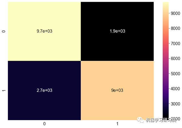
混淆矩阵：

混淆矩阵是一种分类模型的性能测量技术。它是一种表格，有助于了解一组测试数据上的分类模型，因为它们的真实值是已知的。

pred_pb=rf_clf.predict_proba(xc_test)[:,1]
Fpr,Tpr,thresholds = roc_curve(yc_test,pred_pb,pos_label=True)
auc = roc_auc_score(yc_test,pred_pb)
print(" ROC_AUC score is ",auc)
print("accuracy score is : ",accuracy_score(yc_test,yc_pred))
print("Precision is : " ,precision_score(yc_test, yc_pred))
print("Recall is: " ,recall_score(yc_test, yc_pred))
print("F1 Score is : " ,f1_score(yc_test, yc_pred))
print("classification report \n",classification_report(yc_test,yc_pred))
#绘制混淆矩阵
cnf = confusion_matrix(yc_test,yc_pred)
sns.heatmap(cnf, annot=True, cmap = "magma")1.
2.
3.
4.
5.
6.
7.
8.
9.
10.
11.
12.

分类报告：

分类报告是一种性能评估指标。它用于显示训练分类模型的准确率、召回率、F1 分数和支持度。

ROC_AUC score is  0.8804566893762799
accuracy score is :  0.8127466117687425
Precision is :  0.8397949673811743
Recall is:  0.7729456167438669
F1 Score is :  0.8049848132928354
classification report  
           precision  recall  f1-score   support
        0.0    0.79    0.85      0.82     11658
        1.0    0.84    0.77      0.80     11658
   accuracy                      0.81     23316
  macro avg    0.81    0.81      0.81     23316
weighted avg    0.81    0.81      0.81     233161.
2.
3.
4.
5.
6.
7.
8.
9.
10.
11.
12.

AUC_ROC 曲线：

AUC_ROC 曲线是在各种阈值设置下对分类问题的性能测量。ROC 是概率曲线，AUC 表示可分离性的程度或度量。它告诉模型能够在多大程度上区分类别。

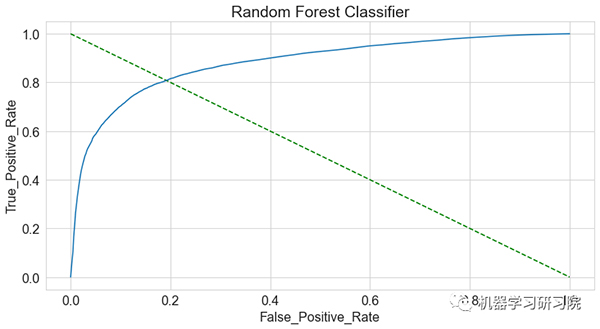
观察得到：

为模型找到了不错的准确度分数(~0.86) 、精确度和召回率。
AUC_ROC 曲线显示了测试值和预测值之间的匹配良好。
总的来说，这表明该模型非常适合预测。

XGBoost 分类器

为了进一步提高预测准确性和 ROC_AUC 分数，尝试使用XGBoost 分类器，因为它本质上非常适合不平衡分类问题。

由于本文篇幅较长，这里省略代码部分，仅显示输出结果。

对于 XGBoost 分类器预测结果，获得较好的 ROC_AUC 分数（约0.87）。同样，为了查看模型性能可视化不同的性能指标。

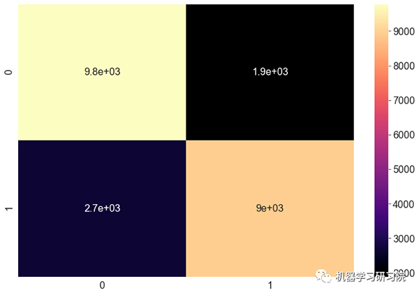
混淆矩阵：

分类报告：

ROC_AUC score is  0.8706238059470456
accuracy score is :  0.8033968090581575
Precision is :  0.8246741325500275
Recall is:  0.7706296105678504
F1 Score is :  0.7967364313586378
classification report  
         precision  recall  f1-score  support
    0.0       0.78    0.84     0.81    11658
    1.0       0.82    0.77     0.80    11658
   accuracy                    0.80     23316
  macro avg   0.80    0.80     0.80    23316
weighted avg   0.80    0.80     0.80    233161.
2.
3.
4.
5.
6.
7.
8.
9.
10.
11.
12.

AUC_ROC 曲线：

观察得到：

绘制的 AUC_ROC 曲线显示测试数据与预测值之间的匹配良好。
发现ROC分数的最大值是0.87。
然而 XGBoost 在测试数据的 AUC 分数下降到约0.86，由此可见出现过度拟合问题。

LGBM 分类模型

为了避免数据集中过度拟合的问题，尝试使用分层 K折交叉验证器并使用 LGBM模型来预测基于分类的概率。

分层 K 折交叉验证器它提供训练/测试索引以将数据拆分为训练/测试集。这个交叉验证对象是 K-Fold 的一种变体，它返回分层折叠。通过保留每个类别的样本百分比来进行折叠。

在这里，我使用了 10 个具有不同参数的分层k折交叉验证。

from lightgbm import LGBMClassifier
lgb_params= {'learning_rate': 0.045,  
            'n_estimators': 10000,
            'max_bin': 84,
            'num_leaves': 10,
            'max_depth': 20,
            'reg_alpha': 8.457,
            'reg_lambda': 6.853,
            'subsample': 0.749}
lgb_model = cross_val(xc, yc,  
              LGBMClassifier,  
             lgb_params)1.
2.
3.
4.
5.
6.
7.
8.
9.
10.
11.
12.

运行LGBM算法后，得到一个不错的 ROC_AUC分数（约0.87）。接下来使用不同指标检验模型性能。

混淆矩阵：

分类报告：

ROC_AUC score is  0.8706238059470456
accuracy score is :  0.8030965860353405
Precision is :  0.8258784469242829
Recall is:  0.7681420483787956
F1 Score is :  0.7959646237944981
classification report  
        precision    recall  f1-score  support
   0.0       0.78      0.84      0.81   11658
   1.0       0.83      0.77      0.80   11658
   accuracy                      0.80   23316
  macro avg  0.80      0.80      0.80   23316
weighted avg  0.80      0.80      0.80   233161.
2.
3.
4.
5.
6.
7.
8.
9.
10.
11.
12.

AUC_ROC 曲线：

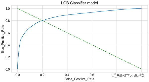
观察得到：

该模型在测试集上表现较好，AUC得分为约0.871。
这样有效地解决了模型过拟合问题。
根据可视化的性能指标，即AUC_ROC曲线，显示了测试值和预测值之间的匹配良好。

模型预测

预测数据集准备

① 可以删除不相关且对数据没有影响的列，例如 "source" 列。

df_3 = df_testdf_3.drop(
         columns=["source"],
         inplace=True)
df_3.head()1.
2.
3.
4.

② 从测试数据集中删除目标变量。

xc_pred = df_3.drop(columns=['Is_Lead',"ID"])1.

③ 使用StandardScaler对 x 的值进行数据标准化，得到呈正态分布的数据集。

sc = StandardScaler()
df_xc_pred = pd.DataFrame(
     sc.fit_transform(xc_pred),
     columns=xc_pred.columns)
Lead_pred_xg=clf2.predict_proba(df_xc_pred)[:,1]
Lead_pred_lgb=lgb_model.predict_proba(df_xc_pred)[:,1]
Lead_pred_rf=rf_clf.predict_proba(df_xc_pred)[:,1]
print(lead_pred_xg,lead_pred_lgb,lead_pred_rf)
[0.09673516 0.9428428  0.12728807 ...  
 0.31698707 0.1821623  0.17593904]  
[0.14278614 0.94357392 0.13603912 ...  
 0.22251432 0.24186564 0.16873483]  
[0.17 0.97 0.09 ...  
0.5  0.09 0.15]1.
2.
3.
4.
5.
6.
7.
8.
9.
10.
11.
12.
13.
14.

④ 为潜在客户预测创建DataFrame数据框。

#用于潜在客户预测的数据框Lead_pred_lgb= pd.DataFrame(lead_pred_lgb,columns=["Is_Lead"])Lead_pred_xg= pd.DataFrame(lead_pred_xg,columns=["Is_Lead"])Lead_pred_rf= pd.DataFrame(lead_pred_rf,columns=["Is_Lead"])1.

⑤ 将"ID"和预测保存到所有模型的 csv 文件中。

#为XG模型保存ID和预测到csv文件
df_pred_xg=pd.concat([df_test["ID"],lead_pred_xg],axis=1,ignore_index=True)
df_pred_xg.columns = ["ID","Is_Lead"]
print(df_pred_xg.head())
df_pred_xg.to_csv("Credit_Card_Lead_Predictions_final_xg.csv",index=False)
#为LGB模型保存ID和预测到csv文件
df_pred_lgb=pd.concat([df_test["ID"],lead_pred_lgb],axis=1,ignore_index=True)
df_pred_lgb.columns = ["ID","Is_Lead"]
print(df_pred_lgb.head())
df_pred_lgb.to_csv("Credit_Card_Lead_Predictions_final_lgb.csv",index=False)
#为RF模型保存ID和预测到csv文件
df_pred_rf=pd.concat([df_test["ID"],lead_pred_rf],axis=1,ignore_index=True)
df_pred_rf.columns = ["ID","Is_Lead"]
print(df_pred_rf.head())
df_pred_rf.to_csv("Credit_Card_Lead_Predictions_final_rf.csv",index=False)1.
2.
3.
4.
5.
6.
7.
8.
9.
10.
11.
12.
13.
14.
15.

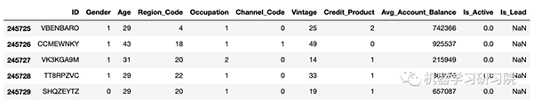
⑥ LGBM 模型输出。

ID   Is_Lead
VBENBARO  0.096735
CCMEWNKY  0.942843
VK3KGA9M  0.127288
TT8RPZVC  0.052260
SHQZEYTZ  0.057762
        ID   Is_Lead
VBENBARO  0.142786
CCMEWNKY  0.943574
VK3KGA9M  0.136039
TT8RPZVC  0.084144
SHQZEYTZ  0.055887
        ID  Is_Lead
VBENBARO     0.17
CCMEWNKY     0.97
VK3KGA9M     0.09
TT8RPZVC     0.12
SHQZEYTZ     0.091.


















因此，LGBM 被选为最终模型，因为该模型在训练集和测试集上均具有最高及最一致的 AUC 分数。

预测模型存储

这里使用joblib库保存模型。

import joblib
# 将模型保存为文件中的pickle
joblib.dump(lgb_model,
          'lgb_model.pkl')
['lgb_model.pkl']1.
2.
3.
4.
5.

写在最后

数据包含分类数据和数值数据。将类别转换为数值数据以进行EDA分析。

还进行了数据可视化分析，并得到到以下情况:

在过去3个月里，与企业家相比，活跃客户更多地来自工薪阶层、个体经营者和其他人群。
目标变量是不平衡的，需要进行样本平衡处理以有效的建模。本案例中利用欠采样技术实现数据集的平衡。

随机森林分类器

发现随机森林模型的AUC得分最高(约0.91)。
然而，随机森林模型在测试数据集上的AUC得分只有约0.85。

XGBoost分类器

为了进一步提高准确率，我们使用 XGBoost 模型，通过训练数据发现AUC得分为0.87。
然而，XGBoost 模型在测试数据集上的 AUC 评分下降到约0.86，存在过拟合问题。

分层交叉验证的LGBM分类器

为解决过拟合问题，采用10折交叉验证的LGBM模型，在训练数据上AUC得分为0.874。
该模型在测试数据上表现同样良好，AUC 得分约 0.871。
因此，我们选择LGBM模型作为最终模型，因为它在训练集和测试集上AUC得分最高，且最一致的。