Python中文社区 (ID:python-china)
某些预测问题需要为同一输入预测数字值和类别标签。一种简单的方法是在同一数据上开发回归和分类预测模型,然后依次使用这些模型。另一种通常更有效的方法是开发单个神经网络模型,该模型可以根据同一输入预测数字和类别标签值。这被称为多输出模型,使用现代深度学习库(例如Keras和TensorFlow)可以相对容易地开发和评估。
在本教程中,您将发现如何开发用于组合回归和分类预测的神经网络。完成本教程后,您将知道:
- 一些预测问题需要为每个输入示例预测数字和类别标签值。
- 如何针对需要多个输出的问题开发单独的回归和分类模型。
- 如何开发和评估能够同时进行回归和分类预测的神经网络模型。
教程概述
本教程分为三个部分:他们是:
- 回归和分类的单一模型
- 单独的回归和分类模型
鲍鱼数据集
回归模型
分类模型
- 组合回归和分类模型
回归和分类的单一模型
开发用于回归或分类问题的深度学习神经网络模型是很常见的,但是在某些预测建模任务上,我们可能希望开发一个可以进行回归和分类预测的单一模型。回归是指涉及预测给定输入的数值的预测建模问题。分类是指预测建模问题,涉及预测给定输入的类别标签或类别标签的概率。
我们可能要预测数值和分类值时可能会有一些问题。解决此问题的一种方法是为每个所需的预测开发一个单独的模型。这种方法的问题在于,由单独的模型做出的预测可能会有所不同。使用神经网络模型时可以使用的另一种方法是开发单个模型,该模型能够对相同输入的数字和类输出进行单独的预测。这称为多输出神经网络模型。这种类型的模型的好处在于,我们有一个模型可以开发和维护,而不是两个模型,并且同时在两种输出类型上训练和更新模型可以在两种输出类型之间的预测中提供更大的一致性。我们将开发一个能够同时进行回归和分类预测的多输出神经网络模型。
首先,让我们选择一个满足此要求的数据集,并从为回归和分类预测开发单独的模型开始。
单独的回归和分类模型
在本节中,我们将从选择一个实际数据集开始,在该数据集中我们可能需要同时进行回归和分类预测,然后针对每种类型的预测开发单独的模型。
鲍鱼数据集
我们将使用“鲍鱼”数据集。确定鲍鱼的年龄是一项耗时的工作,并且希望仅根据物理细节来确定鲍鱼的年龄。这是一个描述鲍鱼物理细节的数据集,需要预测鲍鱼的环数,这是该生物年龄的代名词。
“年龄”既可以预测为数值(以年为单位),也可以预测为类别标签(按年为普通年)。无需下载数据集,因为我们将作为工作示例的一部分自动下载它。数据集提供了一个数据集示例,我们可能需要输入的数值和分类。
首先,让我们开发一个示例来下载和汇总数据集。
- # load and summarize the abalone dataset
- from pandas import read_csv
- from matplotlib import pyplot
- # load dataset
- url = 'https://raw.githubusercontent.com/jbrownlee/Datasets/master/abalone.csv'
- dataframe = read_csv(url, header=None)
- # summarize shape
- print(dataframe.shape)
- # summarize first few lines
- print(dataframe.head())
首先运行示例,然后下载并汇总数据集的形状。我们可以看到有4,177个示例(行)可用于训练和评估模型,还有9个要素(列)包括目标变量。我们可以看到,除了第一个字符串值之外,所有输入变量都是数字变量。为了简化数据准备,我们将从模型中删除第一列,并着重于对数字输入值进行建模。
- (4177, 9)
- 012345678
- 0 M 0.4550.3650.0950.51400.22450.10100.15015
- 1 M 0.3500.2650.0900.22550.09950.04850.0707
- 2 F 0.5300.4200.1350.67700.25650.14150.2109
- 3 M 0.4400.3650.1250.51600.21550.11400.15510
- 4 I 0.3300.2550.0800.20500.08950.03950.0557
我们可以将数据用作开发单独的回归和分类多层感知器(MLP)神经网络模型的基础。
注意:我们并未尝试为此数据集开发最佳模型;相反,我们正在展示一种特定的技术:开发可以进行回归和分类预测的模型。
回归模型
在本节中,我们将为鲍鱼数据集开发回归MLP模型。首先,我们必须将各列分为输入和输出元素,并删除包含字符串值的第一列。我们还将强制所有加载的列都具有浮点类型(由神经网络模型期望)并记录输入特征的数量,稍后模型需要知道这些特征。
- # split into input (X) and output (y) variables
- X, y = dataset[:, 1:-1], dataset[:, -1]
- X, y = X.astype('float'), y.astype('float')
- n_features = X.shape[1]
接下来,我们可以将数据集拆分为训练和测试数据集。我们将使用67%的随机样本来训练模型,而剩余的33%则用于评估模型。
- # split data into train and test sets
- X_train, X_test, y_train, y_test = train_test_split(X, y, test_size=0.33, random_state=1)
然后,我们可以定义一个MLP神经网络模型。该模型将具有两个隐藏层,第一个具有20个节点,第二个具有10个节点,都使用ReLU激活和“正常”权重初始化(一种好的做法)。层数和节点数是任意选择的。输出层将具有用于预测数值和线性激活函数的单个节点。
- # define the keras model
- model = Sequential()
- model.add(Dense(20, input_dim=n_features, activation='relu', kernel_initializer='he_normal'))
- model.add(Dense(10, activation='relu', kernel_initializer='he_normal'))
- model.add(Dense(1, activation='linear'))
使用随机梯度下降的有效Adam版本,将训练模型以最小化均方误差(MSE)损失函数。
- # compile the keras model
- model.compile(loss='mse', optimizer='adam')
我们将训练150个纪元的模型,并以32个样本的小批量为样本,再次任意选择。
- # fit the keras model on the dataset
- model.fit(X_train, y_train, epochs=150, batch_size=32, verbose=2)
最后,在训练完模型后,我们将在保持测试数据集上对其进行评估,并报告平均绝对误差(MAE)。
- # evaluate on test set
- yhat = model.predict(X_test)
- error = mean_absolute_error(y_test, yhat)
- print('MAE: %.3f'% error)
综上所述,下面列出了以回归问题为框架的鲍鱼数据集的MLP神经网络的完整示例。
- # regression mlp model for the abalone dataset
- from pandas import read_csv
- from tensorflow.keras.models importSequential
- from tensorflow.keras.layers importDense
- from sklearn.metrics import mean_absolute_error
- from sklearn.model_selection import train_test_split
- # load dataset
- url = 'https://raw.githubusercontent.com/jbrownlee/Datasets/master/abalone.csv'
- dataframe = read_csv(url, header=None)
- dataset = dataframe.values
- # split into input (X) and output (y) variables
- X, y = dataset[:, 1:-1], dataset[:, -1]
- X, y = X.astype('float'), y.astype('float')
- n_features = X.shape[1]
- # split data into train and test sets
- X_train, X_test, y_train, y_test = train_test_split(X, y, test_size=0.33, random_state=1)
- # define the keras model
- model = Sequential()
- model.add(Dense(20, input_dim=n_features, activation='relu', kernel_initializer='he_normal'))
- model.add(Dense(10, activation='relu', kernel_initializer='he_normal'))
- model.add(Dense(1, activation='linear'))
- # compile the keras model
- model.compile(loss='mse', optimizer='adam')
- # fit the keras model on the dataset
- model.fit(X_train, y_train, epochs=150, batch_size=32, verbose=2)
- # evaluate on test set
- yhat = model.predict(X_test)
- error = mean_absolute_error(y_test, yhat)
- print('MAE: %.3f'% error)
运行示例将准备数据集,拟合模型并报告模型误差的估计值。
注意:由于算法或评估程序的随机性,或者数值精度的差异,您的结果可能会有所不同。考虑运行该示例几次并比较平均结果。
在这种情况下,我们可以看到该模型实现了约1.5 的误差。
- Epoch145/150
- 88/88- 0s- loss: 4.6130
- Epoch146/150
- 88/88- 0s- loss: 4.6182
- Epoch147/150
- 88/88- 0s- loss: 4.6277
- Epoch148/150
- 88/88- 0s- loss: 4.6437
- Epoch149/150
- 88/88- 0s- loss: 4.6166
- Epoch150/150
- 88/88- 0s- loss: 4.6132
- MAE: 1.554
到目前为止,一切都很好。接下来,让我们看一下开发类似的分类模型。
分类模型
鲍鱼数据集可以归类为一个分类问题,其中每个“环”整数都被当作一个单独的类标签。该示例和模型与上述回归示例非常相似,但有一些重要的变化。这要求首先为每个“ ring”值分配一个单独的整数,从0开始,以“ class”总数减1结束。这可以使用LabelEncoder实现。我们还可以将类的总数记录为唯一编码的类值的总数,稍后模型会需要。
- # encode strings to integer
- y = LabelEncoder().fit_transform(y)
- n_class = len(unique(y))
将数据像以前一样分为训练集和测试集后,我们可以定义模型并将模型的输出数更改为等于类数,并使用对于多类分类通用的softmax激活函数。
- # define the keras model
- model = Sequential()
- model.add(Dense(20, input_dim=n_features, activation='relu', kernel_initializer='he_normal'))
- model.add(Dense(10, activation='relu', kernel_initializer='he_normal'))
- model.add(Dense(n_class, activation='softmax'))
假设我们已将类别标签编码为整数值,则可以通过最小化适用于具有整数编码类别标签的多类别分类任务的稀疏类别交叉熵损失函数来拟合模型
- # compile the keras model
- model.compile(loss='sparse_categorical_crossentropy', optimizer='adam')
在像以前一样将模型拟合到训练数据集上之后,我们可以通过计算保留测试集上的分类准确性来评估模型的性能。
- # evaluate on test set
- yhat = model.predict(X_test)
- yhat = argmax(yhat, axis=-1).astype('int')
- acc = accuracy_score(y_test, yhat)
- print('Accuracy: %.3f'% acc)
综上所述,下面列出了针对鲍鱼数据集的MLP神经网络的完整示例,该示例被归类为分类问题。
- # classification mlp model for the abalone dataset
- from numpy import unique
- from numpy import argmax
- from pandas import read_csv
- from tensorflow.keras.models importSequential
- from tensorflow.keras.layers importDense
- from sklearn.metrics import accuracy_score
- from sklearn.model_selection import train_test_split
- from sklearn.preprocessing importLabelEncoder
- # load dataset
- url = 'https://raw.githubusercontent.com/jbrownlee/Datasets/master/abalone.csv'
- dataframe = read_csv(url, header=None)
- dataset = dataframe.values
- # split into input (X) and output (y) variables
- X, y = dataset[:, 1:-1], dataset[:, -1]
- X, y = X.astype('float'), y.astype('float')
- n_features = X.shape[1]
- # encode strings to integer
- y = LabelEncoder().fit_transform(y)
- n_class = len(unique(y))
- # split data into train and test sets
- X_train, X_test, y_train, y_test = train_test_split(X, y, test_size=0.33, random_state=1)
- # define the keras model
- model = Sequential()
- model.add(Dense(20, input_dim=n_features, activation='relu', kernel_initializer='he_normal'))
- model.add(Dense(10, activation='relu', kernel_initializer='he_normal'))
- model.add(Dense(n_class, activation='softmax'))
- # compile the keras model
- model.compile(loss='sparse_categorical_crossentropy', optimizer='adam')
- # fit the keras model on the dataset
- model.fit(X_train, y_train, epochs=150, batch_size=32, verbose=2)
- # evaluate on test set
- yhat = model.predict(X_test)
- yhat = argmax(yhat, axis=-1).astype('int')
- acc = accuracy_score(y_test, yhat)
- print('Accuracy: %.3f'% acc)
运行示例将准备数据集,拟合模型并报告模型误差的估计值。
注意:由于算法或评估程序的随机性,或者数值精度的差异,您的结果可能会有所不同。考虑运行该示例几次并比较平均结果。
在这种情况下,我们可以看到该模型的准确度约为27%。
- Epoch145/150
- 88/88- 0s- loss: 1.9271
- Epoch146/150
- 88/88- 0s- loss: 1.9265
- Epoch147/150
- 88/88- 0s- loss: 1.9265
- Epoch148/150
- 88/88- 0s- loss: 1.9271
- Epoch149/150
- 88/88- 0s- loss: 1.9262
- Epoch150/150
- 88/88- 0s- loss: 1.9260
- Accuracy: 0.274
到目前为止,一切都很好。接下来,让我们看一下开发一种能够同时进行回归和分类预测的组合模型。
组合回归和分类模型
在本节中,我们可以开发一个单一的MLP神经网络模型,该模型可以对单个输入进行回归和分类预测。这称为多输出模型,可以使用功能性Keras API进行开发。
首先,必须准备数据集。尽管我们应该使用单独的名称保存编码后的目标变量以将其与原始目标变量值区分开,但是我们可以像以前一样为分类准备数据集。
- # encode strings to integer
- y_class = LabelEncoder().fit_transform(y)
- n_class = len(unique(y_class))
然后,我们可以将输入,原始输出和编码后的输出变量拆分为训练集和测试集。
- # split data into train and test sets
- X_train, X_test, y_train, y_test, y_train_class, y_test_class = train_test_split(X, y, y_class, test_size=0.33, random_state=1)
接下来,我们可以使用功能性API定义模型。该模型采用与独立模型相同的输入数量,并使用以相同方式配置的两个隐藏层
- # input
- visible = Input(shape=(n_features,))
- hidden1 = Dense(20, activation='relu', kernel_initializer='he_normal')(visible)
- hidden2 = Dense(10, activation='relu', kernel_initializer='he_normal')(hidden1)
然后,我们可以定义两个单独的输出层,它们连接到模型的第二个隐藏层。
第一个是具有单个节点和线性激活函数的回归输出层。
- # regression output
- out_reg = Dense(1, activation='linear')(hidden2)
第二个是分类输出层,对于每个要预测的类都有一个节点,并使用softmax激活函数。
- # classification output
- out_clas = Dense(n_class, activation='softmax')(hidden2)
然后,我们可以使用一个输入层和两个输出层定义模型。
- # define model
- model = Model(inputs=visible, outputs=[out_reg, out_clas])
给定两个输出层,我们可以使用两个损失函数来编译模型,第一个(回归)输出层的均方误差损失和第二个(分类)输出层的稀疏分类交叉熵。
- # compile the keras model
- model.compile(loss=['mse','sparse_categorical_crossentropy'], optimizer='adam')
我们还可以创建模型图以供参考。这需要安装pydot和pygraphviz。如果存在问题,则可以注释掉该行以及 plot_model()函数的import语句。
- # plot graph of model
- plot_model(model, to_file='model.png', show_shapes=True)
每次模型进行预测时,它将预测两个值。同样,训练模型时,每个输出每个样本将需要一个目标变量。这样,我们可以训练模型,并仔细地向模型的每个输出提供回归目标和分类目标数据。
- # plot graph of model
- plot_model(model, to_file='model.png', show_shapes=True)
然后,拟合模型可以对保留测试集中的每个示例进行回归和分类预测。
- # make predictions on test set
- yhat1, yhat2 = model.predict(X_test)
第一个数组可用于通过平均绝对误差评估回归预测。
- # calculate error for regression model
- error = mean_absolute_error(y_test, yhat1)
- print('MAE: %.3f'% error)
第二个数组可用于通过分类准确性评估分类预测。
- # evaluate accuracy for classification model
- yhat2 = argmax(yhat2, axis=-1).astype('int')
- acc = accuracy_score(y_test_class, yhat2)
- print('Accuracy: %.3f'% acc)
就是这样。结合在一起,下面列出了训练和评估用于鲍鱼数据集上的组合器回归和分类预测的多输出模型的完整示例。
- # mlp for combined regression and classification predictions on the abalone dataset
- from numpy import unique
- from numpy import argmax
- from pandas import read_csv
- from sklearn.metrics import mean_absolute_error
- from sklearn.metrics import accuracy_score
- from sklearn.model_selection import train_test_split
- from sklearn.preprocessing importLabelEncoder
- from tensorflow.keras.models importModel
- from tensorflow.keras.layers importInput
- from tensorflow.keras.layers importDense
- from tensorflow.keras.utils import plot_model
- # load dataset
- url = 'https://raw.githubusercontent.com/jbrownlee/Datasets/master/abalone.csv'
- dataframe = read_csv(url, header=None)
- dataset = dataframe.values
- # split into input (X) and output (y) variables
- X, y = dataset[:, 1:-1], dataset[:, -1]
- X, y = X.astype('float'), y.astype('float')
- n_features = X.shape[1]
- # encode strings to integer
- y_class = LabelEncoder().fit_transform(y)
- n_class = len(unique(y_class))
- # split data into train and test sets
- X_train, X_test, y_train, y_test, y_train_class, y_test_class = train_test_split(X, y, y_class, test_size=0.33, random_state=1)
- # input
- visible = Input(shape=(n_features,))
- hidden1 = Dense(20, activation='relu', kernel_initializer='he_normal')(visible)
- hidden2 = Dense(10, activation='relu', kernel_initializer='he_normal')(hidden1)
- # regression output
- out_reg = Dense(1, activation='linear')(hidden2)
- # classification output
- out_clas = Dense(n_class, activation='softmax')(hidden2)
- # define model
- model = Model(inputs=visible, outputs=[out_reg, out_clas])
- # compile the keras model
- model.compile(loss=['mse','sparse_categorical_crossentropy'], optimizer='adam')
- # plot graph of model
- plot_model(model, to_file='model.png', show_shapes=True)
- # fit the keras model on the dataset
- model.fit(X_train, [y_train,y_train_class], epochs=150, batch_size=32, verbose=2)
- # make predictions on test set
- yhat1, yhat2 = model.predict(X_test)
- # calculate error for regression model
- error = mean_absolute_error(y_test, yhat1)
- print('MAE: %.3f'% error)
- # evaluate accuracy for classification model
- yhat2 = argmax(yhat2, axis=-1).astype('int')
- acc = accuracy_score(y_test_class, yhat2)
- print('Accuracy: %.3f'% acc)
运行示例将准备数据集,拟合模型并报告模型误差的估计值。
注意:由于算法或评估程序的随机性,或者数值精度的差异,您的结果可能会有所不同。考虑运行该示例几次并比较平均结果。
创建了多输出模型图,清楚地显示了连接到模型第二个隐藏层的回归(左)和分类(右)输出层。
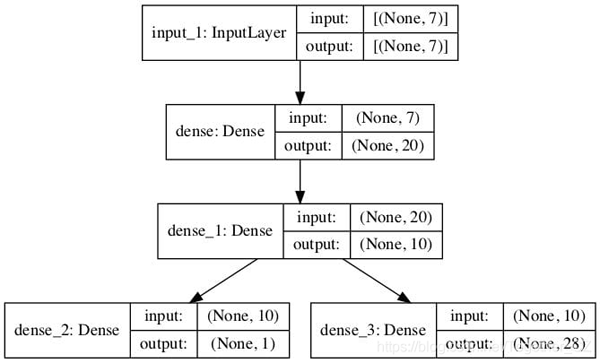
在这种情况下,我们可以看到该模型既实现了约1.495 的合理误差,又实现了与之前相似的约25.6%的精度。
- Epoch145/150
- 88/88- 0s- loss: 6.5707- dense_2_loss: 4.5396- dense_3_loss: 2.0311
- Epoch146/150
- 88/88- 0s- loss: 6.5753- dense_2_loss: 4.5466- dense_3_loss: 2.0287
- Epoch147/150
- 88/88- 0s- loss: 6.5970- dense_2_loss: 4.5723- dense_3_loss: 2.0247
- Epoch148/150
- 88/88- 0s- loss: 6.5640- dense_2_loss: 4.5389- dense_3_loss: 2.0251
- Epoch149/150
- 88/88- 0s- loss: 6.6053- dense_2_loss: 4.5827- dense_3_loss: 2.0226
- Epoch150/150
- 88/88- 0s- loss: 6.5754- dense_2_loss: 4.5524- dense_3_loss: 2.0230
- MAE: 1.495
- Accuracy: 0.256