XGBoost是梯度分类和回归问题的有效实现。
它既快速又高效,即使在各种预测建模任务上也表现出色,即使不是最好的,也能在数据科学竞赛的获胜者(例如Kaggle的获奖者)中广受青睐。
XGBoost也可以用于时间序列预测,尽管它要求将时间序列数据集首先转换为有监督的学习问题。它还需要使用一种专门的技术来评估模型,称为前向验证,因为使用k倍交叉验证对模型进行评估会导致乐观的结果。
在本教程中,您将发现如何开发XGBoost模型进行时间序列预测。完成本教程后,您将知道:
1、XGBoost是用于分类和回归的梯度提升集成算法的实现。
2、可以使用滑动窗口表示将时间序列数据集转换为监督学习。
3、如何使用XGBoost模型拟合,评估和进行预测,以进行时间序列预测。
教程概述
本教程分为三个部分:他们是:
1、XGBoost集成
2、时间序列数据准备
3、XGBoost用于时间序列预测
XGBoost集成
XGBoost是Extreme Gradient Boosting的缩写,是随机梯度提升机器学习算法的有效实现。随机梯度增强算法(也称为梯度增强机或树增强)是一种功能强大的机器学习技术,可在各种具有挑战性的机器学习问题上表现出色,甚至表现最佳。
它是决策树算法的集合,其中新树修复了那些已经属于模型的树的错误。将添加树,直到无法对模型进行进一步的改进为止。XGBoost提供了随机梯度提升算法的高效实现,并提供了一组模型超参数,这些参数旨在提供对模型训练过程的控制。
XGBoost设计用于表格数据集的分类和回归,尽管它可以用于时间序列预测。
首先,必须安装XGBoost库。您可以使用pip进行安装,如下所示:
- sudo pip install xgboost
一旦安装,您可以通过运行以下代码来确认它已成功安装,并且您正在使用现代版本:
- # xgboost
- import xgboost
- print("xgboost", xgboost.__version__)
运行代码,您应该看到以下版本号或更高版本。
- xgboost 1.0.1
尽管XGBoost库具有自己的Python API,但我们可以通过XGBRegressor包装器类将XGBoost模型与scikit-learn API结合使用。
可以实例化模型的实例,就像将其用于模型评估的任何其他scikit-learn类一样使用。例如:
- # define model
- model = XGBRegressor()
现在我们已经熟悉了XGBoost,下面让我们看一下如何为监督学习准备时间序列数据集。
时间序列数据准备
时间序列数据可以表述为监督学习。给定时间序列数据集的数字序列,我们可以将数据重组为看起来像监督学习的问题。我们可以通过使用以前的时间步长作为输入变量,并使用下一个时间步长作为输出变量来做到这一点。让我们通过一个例子来具体说明。假设我们有一个时间序列,如下所示:
- time, measure
- 1, 100
- 2, 110
- 3, 108
- 4, 115
- 5, 120
通过使用上一个时间步的值来预测下一个时间步的值,我们可以将此时间序列数据集重组为监督学习问题。通过这种方式重组时间序列数据集,数据将如下所示:
- X, y
- ?, 100
- 100, 110
- 110, 108
- 108, 115
- 115, 120
- 120, ?
请注意,时间列已删除,某些数据行不可用于训练模型,例如第一和最后一个。
这种表示称为滑动窗口,因为输入和预期输出的窗口会随着时间向前移动,从而为监督学习模型创建新的“样本”。
有关准备时间序列预测数据的滑动窗口方法的更多信息。
在给定所需的输入和输出序列长度的情况下,我们可以在Pandas中使用shift()函数自动创建时间序列问题的新框架。
这将是一个有用的工具,因为它将允许我们使用机器学习算法探索时间序列问题的不同框架,以查看可能导致性能更好的模型。
下面的函数将一个时间序列作为具有一个或多个列的NumPy数组时间序列,并将其转换为具有指定数量的输入和输出的监督学习问题。
- # transform a time series dataset into a supervised learning dataset
- def series_to_supervised(data, n_in=1, n_out=1, dropnan=True):
- n_vars = 1 if type(data) is list else data.shape[1]
- df = DataFrame(data)
- cols = list()
- # input sequence (t-n, ... t-1)
- for i in range(n_in, 0, -1):
- cols.append(df.shift(i))
- # forecast sequence (t, t+1, ... t+n)
- for i in range(0, n_out):
- cols.append(df.shift(-i))
- # put it all together
- agg = concat(cols, axis=1)
- # drop rows with NaN values
- if dropnan:
- agg.dropna(inplace=True)
- return agg.values
我们可以使用此函数为XGBoost准备时间序列数据集。
准备好数据集后,我们必须小心如何使用它来拟合和评估模型。
例如,将模型拟合未来的数据并预测过去是无效的。该模型必须在过去进行训练并预测未来。这意味着不能使用在评估过程中将数据集随机化的方法,例如k折交叉验证。相反,我们必须使用一种称为前向验证的技术。在前向验证中,首先通过选择一个切点(例如除过去12个月外,所有数据均用于培训,最近12个月用于测试。
如果我们有兴趣进行单步预测,例如一个月后,我们可以通过对训练数据集进行训练并预测测试数据集的第一步来评估模型。然后,我们可以将来自测试集的真实观测值添加到训练数据集中,重新拟合模型,然后让模型预测测试数据集中的第二步。对整个测试数据集重复此过程将为整个测试数据集提供一步式预测,可以从中计算出误差度量以评估模型的技能。
下面的函数执行前向验证。它使用时间序列数据集的整个监督学习版本以及用作测试集的行数作为参数。然后,它逐步通过测试集,调用xgboost_forecast()函数进行单步预测。计算错误度量,并将详细信息返回以进行分析。
- # walk-forward validation for univariate data
- def walk_forward_validation(data, n_test):
- predictions = list()
- # split dataset
- train, test = train_test_split(data, n_test)
- # seed history with training dataset
- history = [x for x in train]
- # step over each time-step in the test set
- for i in range(len(test)):
- # split test row into input and output columns
- testX, testtesty = test[i, :-1], test[i, -1]
- # fit model on history and make a prediction
- yhat = xgboost_forecast(history, testX)
- # store forecast in list of predictions
- predictions.append(yhat)
- # add actual observation to history for the next loop
- history.append(test[i])
- # summarize progress
- print('>expected=%.1f, predicted=%.1f' % (testy, yhat))
- # estimate prediction error
- error = mean_absolute_error(test[:, -1], predictions)
- return error, test[:, 1], predictions
调用train_test_split()函数可将数据集拆分为训练集和测试集。我们可以在下面定义此功能。
- # split a univariate dataset into train/test sets
- def train_test_split(data, n_test):
- return data[:-n_test, :], data[-n_test:, :]
我们可以使用XGBRegressor类进行单步预测。下面的xgboost_forecast()函数通过将训练数据集和测试输入行作为输入,拟合模型并进行单步预测来实现此目的。
- # fit an xgboost model and make a one step prediction
- def xgboost_forecast(train, testX):
- # transform list into array
- train = asarray(train)
- # split into input and output columns
- trainX, traintrainy = train[:, :-1], train[:, -1]
- # fit model
- model = XGBRegressor(objective='reg:squarederror', n_estimators=1000)
- model.fit(trainX, trainy)
- # make a one-step prediction
- yhat = model.predict([testX])
- return yhat[0]
现在,我们知道了如何准备时间序列数据以进行预测和评估XGBoost模型,接下来我们可以看看在实际数据集上使用XGBoost的情况。
XGBoost用于时间序列预测
在本节中,我们将探索如何使用XGBoost进行时间序列预测。我们将使用标准的单变量时间序列数据集,以使用该模型进行单步预测。您可以将本节中的代码用作您自己项目的起点,并轻松地对其进行调整以适应多变量输入,多变量预测和多步预测。我们将使用每日女性出生数据集,即三年中的每月出生数。
您可以从此处下载数据集,并将其放在文件名“ daily-total-female-births.csv”的当前工作目录中。
数据集(每天女性出生总数.csv):
- https://raw.githubusercontent.com/jbrownlee/Datasets/master/daily-total-female-births.csv
说明(每日女性出生总数):
- https://raw.githubusercontent.com/jbrownlee/Datasets/master/daily-total-female-births.names
数据集的前几行如下所示:
- "Date","Births"
- "1959-01-01",35
- "1959-01-02",32
- "1959-01-03",30
- "1959-01-04",31
- "1959-01-05",44
- ...
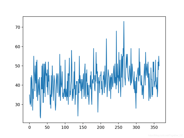
首先,让我们加载并绘制数据集。下面列出了完整的示例。
- # load and plot the time series dataset
- from pandas import read_csv
- from matplotlib import pyplot
- # load dataset
- series = read_csv('daily-total-female-births.csv', header=0, index_col=0)
- values = series.values
- # plot dataset
- pyplot.plot(values)
- pyplot.show()
运行示例将创建数据集的折线图。我们可以看到没有明显的趋势或季节性。
当预测最近的12个月时,持久性模型可以实现约6.7例出生的MAE。这提供了性能基准,在该基准之上可以认为模型是熟练的。
接下来,当对过去12个月的数据进行单步预测时,我们可以评估数据集上的XGBoost模型。
我们将仅使用前6个时间步长作为模型和默认模型超参数的输入,除了我们将损失更改为'reg:squarederror'(以避免警告消息),并在集合中使用1,000棵树(以避免学习不足) )。
下面列出了完整的示例。
- # forecast monthly births with xgboost
- from numpy import asarray
- from pandas import read_csv
- from pandas import DataFrame
- from pandas import concat
- from sklearn.metrics import mean_absolute_error
- from xgboost import XGBRegressor
- from matplotlib import pyplot
- # transform a time series dataset into a supervised learning dataset
- def series_to_supervised(data, n_in=1, n_out=1, dropnan=True):
- n_vars = 1 if type(data) is list else data.shape[1]
- df = DataFrame(data)
- cols = list()
- # input sequence (t-n, ... t-1)
- for i in range(n_in, 0, -1):
- cols.append(df.shift(i))
- # forecast sequence (t, t+1, ... t+n)
- for i in range(0, n_out):
- cols.append(df.shift(-i))
- # put it all together
- agg = concat(cols, axis=1)
- # drop rows with NaN values
- if dropnan:
- agg.dropna(inplace=True)
- return agg.values
- # split a univariate dataset into train/test sets
- def train_test_split(data, n_test):
- return data[:-n_test, :], data[-n_test:, :]
- # fit an xgboost model and make a one step prediction
- def xgboost_forecast(train, testX):
- # transform list into array
- train = asarray(train)
- # split into input and output columns
- trainX, traintrainy = train[:, :-1], train[:, -1]
- # fit model
- model = XGBRegressor(objective='reg:squarederror', n_estimators=1000)
- model.fit(trainX, trainy)
- # make a one-step prediction
- yhat = model.predict(asarray([testX]))
- return yhat[0]
- # walk-forward validation for univariate data
- def walk_forward_validation(data, n_test):
- predictions = list()
- # split dataset
- train, test = train_test_split(data, n_test)
- # seed history with training dataset
- history = [x for x in train]
- # step over each time-step in the test set
- for i in range(len(test)):
- # split test row into input and output columns
- testX, testtesty = test[i, :-1], test[i, -1]
- # fit model on history and make a prediction
- yhat = xgboost_forecast(history, testX)
- # store forecast in list of predictions
- predictions.append(yhat)
- # add actual observation to history for the next loop
- history.append(test[i])
- # summarize progress
- print('>expected=%.1f, predicted=%.1f' % (testy, yhat))
- # estimate prediction error
- error = mean_absolute_error(test[:, -1], predictions)
- return error, test[:, -1], predictions
- # load the dataset
- series = read_csv('daily-total-female-births.csv', header=0, index_col=0)
- values = series.values
- # transform the time series data into supervised learning
- data = series_to_supervised(values, n_in=6)
- # evaluate
- mae, y, yhat = walk_forward_validation(data, 12)
- print('MAE: %.3f' % mae)
- # plot expected vs preducted
- pyplot.plot(y, label='Expected')
- pyplot.plot(yhat, label='Predicted')
- pyplot.legend()
- pyplot.show()
运行示例将报告测试集中每个步骤的期望值和预测值,然后报告所有预测值的MAE。
注意:由于算法或评估程序的随机性,或者数值精度的差异,您的结果可能会有所不同。考虑运行该示例几次并比较平均结果。
我们可以看到,该模型的性能优于持久性模型,MAE约为5.9,而MAE约为6.7
- >expected=42.0, predicted=44.5
- >expected=53.0, predicted=42.5
- >expected=39.0, predicted=40.3
- >expected=40.0, predicted=32.5
- >expected=38.0, predicted=41.1
- >expected=44.0, predicted=45.3
- >expected=34.0, predicted=40.2
- >expected=37.0, predicted=35.0
- >expected=52.0, predicted=32.5
- >expected=48.0, predicted=41.4
- >expected=55.0, predicted=46.6
- >expected=50.0, predicted=47.2
- MAE: 5.957
创建线图,比较数据集最后12个月的一系列期望值和预测值。这给出了模型在测试集上执行得如何的几何解释。
图2
一旦选择了最终的XGBoost模型配置,就可以最终确定模型并用于对新数据进行预测。这称为样本外预测,例如 超出训练数据集进行预测。这与在模型评估期间进行预测是相同的:因为我们始终希望使用模型用于对新数据进行预测时所期望使用的相同过程来评估模型。下面的示例演示了在所有可用数据上拟合最终XGBoost模型并在数据集末尾进行单步预测的过程。
- # finalize model and make a prediction for monthly births with xgboost
- from numpy import asarray
- from pandas import read_csv
- from pandas import DataFrame
- from pandas import concat
- from xgboost import XGBRegressor
- # transform a time series dataset into a supervised learning dataset
- def series_to_supervised(data, n_in=1, n_out=1, dropnan=True):
- n_vars = 1 if type(data) is list else data.shape[1]
- df = DataFrame(data)
- cols = list()
- # input sequence (t-n, ... t-1)
- for i in range(n_in, 0, -1):
- cols.append(df.shift(i))
- # forecast sequence (t, t+1, ... t+n)
- for i in range(0, n_out):
- cols.append(df.shift(-i))
- # put it all together
- agg = concat(cols, axis=1)
- # drop rows with NaN values
- if dropnan:
- agg.dropna(inplace=True)
- return agg.values
- # load the dataset
- series = read_csv('daily-total-female-births.csv', header=0, index_col=0)
- values = series.values
- # transform the time series data into supervised learning
- train = series_to_supervised(values, n_in=6)
- # split into input and output columns
- trainX, traintrainy = train[:, :-1], train[:, -1]
- # fit model
- model = XGBRegressor(objective='reg:squarederror', n_estimators=1000)
- model.fit(trainX, trainy)
- # construct an input for a new preduction
- row = values[-6:].flatten()
- # make a one-step prediction
- yhat = model.predict(asarray([row]))
- print('Input: %s, Predicted: %.3f' % (row, yhat[0]))
运行示例将XGBoost模型适合所有可用数据。使用最近6个月的已知数据准备新的输入行,并预测数据集结束后的下个月。
- Input: [34 37 52 48 55 50], Predicted: 42.708