当我要求你解释文本数据时,你会怎幺做?你将采取什幺步骤来构建文本可视化?
本文将帮助你获得构建可视化和解释文本数据所需的信息。
从文本数据中获得的见解将有助于我们发现文章之间的联系。它将检测趋势和模式。对文本数据的分析将排除噪音,发现以前未知的信息。
这种分析过程也称为探索性文本分析(ETA)。运用K-means、Tf-IDF、词频等方法对这些文本数据进行分析。此外,ETA在数据清理过程中也很有用。
我们还使用Matplotlib、seaborn和Plotly库将结果可视化到图形、词云和绘图中。
在分析文本数据之前,请完成这些预处理任务。
从数据源检索数据
有很多非结构化文本数据可供分析。你可以从以下来源获取数据。
- 来自Kaggle的Twitter文本数据集。
- Reddit和twitter数据集使用API。
- 使用Beautifulsoup从网站上获取文章、。
我将使用路透社的SGML格式的文章。为了便于分析,我将使用beauthoulsoup库从数据文件中获取日期、标题和文章正文。
使用下面的代码从所有数据文件中获取数据,并将输出存储在单个CSV文件中。
- from bs4 import BeautifulSoup
- import pandas as pd
- import csv
- article_dict = {}
- i = 0
- list_of_data_num = []
- for j in range(0,22):
- if j < 10:
- list_of_data_num.append("00" + str(j))
- else:
- list_of_data_num.append("0" + str(j))
- # 循环所有文章以提取日期、标题和文章主体
- for num in list_of_data_num:
- try:
- soup = BeautifulSoup(open("data/reut2-" + num + ".sgm"), features='lxml')
- except:
- continue
- print(num)
- data_reuters = soup.find_all('reuters')
- for data in data_reuters:
- article_dict[i] = {}
- for date in data.find_all('date'):
- try:
- article_dict[i]["date"] = str(date.contents[0]).strip()
- except:
- article_dict[i]["date"] = None
- # print(date.contents[0])
- for title in data.find_all('title'):
- article_dict[i]["title"] = str(title.contents[0]).strip()
- # print(title.contents)
- for text in data.find_all('text'):
- try:
- article_dict[i]["text"] = str(text.contents[4]).strip()
- except:
- article_dict[i]["text"] = None
- i += 1
- dataframe_article = pd.DataFrame(article_dict).T
- dataframe_article.to_csv('articles_data.csv', header=True, index=False, quoting=csv.QUOTE_ALL)
- print(dataframe_article)
还可以使用Regex和OS库组合或循环所有数据文件。
每篇文章的正文以<Reuters>开头,因此使用find_all(‘reuters’)。
你也可以使用pickle模块来保存数据,而不是CSV。
清洗数据
在本节中,我们将从文本数据中移除诸如空值、标点符号、数字等噪声。首先,我们删除文本列中包含空值的行。然后我们处理另一列的空值。
- import pandas as pd import re
- articles_data = pd.read_csv(‘articles_data.csv’) print(articles_data.apply(lambda x: sum(x.isnull()))) articles_nonNull = articles_data.dropna(subset=[‘text’]) articles_nonNull.reset_index(inplace=True)
- def clean_text(text):
- ‘’’Make text lowercase, remove text in square brackets,remove \n,remove punctuation and remove words containing numbers.’’’
- text = str(text).lower()
- text = re.sub(‘<.*?>+’, ‘’, text)
- text = re.sub(‘[%s]’ % re.escape(string.punctuation), ‘’, text)
- text = re.sub(‘\n’, ‘’, text)
- text = re.sub(‘\w*\d\w*’, ‘’, text)
- return text
- articles_nonNull[‘text_clean’]=articles_nonNull[‘text’]\
- .apply(lambda x:clean_text(x))
articles_data = pd.read_csv(‘articles_data.csv’) print(articles_data.apply(lambda x: sum(x.isnull()))) articles_nonNull = articles_data.dropna(subset=[‘text’]) articles_nonNull.reset_index(inplace=True)
def clean_text(text):
‘’’Make text lowercase, remove text in square brackets,remove \n,remove punctuation and remove words containing numbers.’’’
text = str(text).lower()
text = re.sub(‘<.*?>+’, ‘’, text)
text = re.sub(‘[%s]’ % re.escape(string.punctuation), ‘’, text)
text = re.sub(‘\n’, ‘’, text)
text = re.sub(‘\w*\d\w*’, ‘’, text)
return text
articles_nonNull[‘text_clean’]=articles_nonNull[‘text’]\
.apply(lambda x:clean_text(x))
当我们删除文本列中的空值时,其他列中的空值也会消失。
我们使用re方法去除文本数据中的噪声。
数据清理过程中采取的步骤可能会根据文本数据增加或减少。因此,请仔细研究你的文本数据并相应地构建clean_text()方法。
随着预处理任务的完成,我们将继续分析文本数据。
让我们从分析开始。
1.路透社文章篇幅
我们知道所有文章的篇幅不一样。因此,我们将考虑长度等于或超过一段的文章。根据研究,一个句子的平均长度是15-20个单词。一个段落应该有四个句子。
- articles_nonNull[‘word_length’] = articles_nonNull[‘text’].apply(lambda x: len(str(x).split())) print(articles_nonNull.describe())
- articles_word_limit = articles_nonNull[articles_nonNull[‘word_length’] > 60]
- plt.figure(figsize=(12,6))
- p1=sns.kdeplot(articles_word_limit[‘word_length’], shade=True, color=”r”).set_title(‘Kernel Distribution of Number Of words’)
我删除了那些篇幅不足60字的文章。
字长分布是右偏的。
大多数文章有150字左右。
包含事实或股票信息的路透社文章用词较少。
2.路透社文章中的常用词
在这一部分中,我们统计了文章中出现的字数,并对结果进行了分析。我们基于N-gram方法对词数进行了分析。N-gram是基于N值的单词的出现。
我们将从文本数据中删除停用词。因为停用词是噪音,在分析中没有太大用处。
(1)最常见的单字单词(N=1)
让我们在条形图中绘制unigram单词,并为unigram单词绘制词云。
- from gensim.parsing.preprocessing
- import remove_stopwords
- import genism
- from wordcloud import WordCloud
- import numpy as np
- import random
- # 从gensim方法导入stopwords到stop_list变量
- # 你也可以手动添加stopwords
- gensim_stopwords = gensim.parsing.preprocessing.STOPWORDS
- stopwords_list = list(set(gensim_stopwords))
- stopwords_update = ["mln", "vs","cts","said","billion","pct","dlrs","dlr"]
- stopwords = stopwords_list + stopwords_update
- articles_word_limit['temp_list'] = articles_word_limit['text_clean'].apply(lambda x:str(x).split())
- # 从文章中删除停用词
- def remove_stopword(x):
- return [word for word in x if word not in stopwords]
- articles_word_limit['temp_list_stopw'] = articles_word_limit['temp_list'].apply(lambda x:remove_stopword(x))
- # 生成ngram的单词
- def generate_ngrams(text, n_gram=1):
- ngrams = zip(*[text[i:] for i in range(n_gram)])
- return [' '.join(ngram) for ngram in ngrams]
- article_unigrams = defaultdict(int)
- for tweet in articles_word_limit['temp_list_stopw']:
- for word in generate_ngrams(tweet):
- article_unigrams[word] += 1
- article_unigrams_df = pd.DataFrame(sorted(article_unigrams.items(), key=lambda x: x[1])[::-1])
- N=50
- # 在路透社的文章中前50个常用的unigram
- fig, axes = plt.subplots(figsize=(18, 50))
- plt.tight_layout()
- sns.barplot(y=article_unigrams_df[0].values[:N], x=article_unigrams_df[1].values[:N], color='red')
- axes.spines['right'].set_visible(False)
- axes.set_xlabel('')
- axes.set_ylabel('')
- axes.tick_params(axis='x', labelsize=13)
- axes.tick_params(axis='y', labelsize=13)
- axes.set_title(f'Top {N} most common unigrams in Reuters Articles', fontsize=15)
- plt.show()
- # 画出词云
- def col_func(word, font_size, position, orientation, font_path, random_state):
- colors = ['#b58900', '#cb4b16', '#dc322f', '#d33682', '#6c71c4',
- '#268bd2', '#2aa198', '#859900']
- return random.choice(colors)
- fd = {
- 'fontsize': '32',
- 'fontweight' : 'normal',
- 'verticalalignment': 'baseline',
- 'horizontalalignment': 'center',
- }
- wc = WordCloud(width=2000, height=1000, collocations=False,
- background_color="white",
- color_func=col_func,
- max_words=200,
- random_state=np.random.randint(1, 8)) .generate_from_frequencies(article_unigrams)
- fig, ax = plt.subplots(figsize=(20,10))
- ax.imshow(wc, interpolation='bilinear')
- ax.axis("off")
- ax.set_title(‘Unigram Words of Reuters Articles’, pad=24, fontdict=fd)
- plt.show()
Share, trade, stock是一些最常见的词汇,它们是基于股票市场和金融行业的文章。
因此,我们可以说,大多数路透社文章属于金融和股票类。
(2)最常见的Bigram词(N=2)
让我们为Bigram单词绘制条形图和词云。
- article_bigrams = defaultdict(int)
- for tweet in articles_word_limit[‘temp_list_stopw’]:
- for word in generate_ngrams(tweet, n_gram=2):
- article_bigrams[word] += 1
- df_article_bigrams=pd.DataFrame(sorted(article_bigrams.items(),
- key=lambda x: x[1])[::-1])
- N=50
- # 前50个单词的柱状图
- fig, axes = plt.subplots(figsize=(18, 50), dpi=100)
- plt.tight_layout()
- sns.barplot(y=df_article_bigrams[0].values[:N],
- x=df_article_bigrams[1].values[:N],
- color=’red’)
- axes.spines[‘right’].set_visible(False)
- axes.set_xlabel(‘’)
- axes.set_ylabel(‘’)
- axes.tick_params(axis=’x’, labelsize=13)
- axes.tick_params(axis=’y’, labelsize=13)
- axes.set_title(f’Top {N} most common Bigrams in Reuters Articles’,
- fontsize=15)
- plt.show()
- #词云
- wc = WordCloud(width=2000, height=1000, collocations=False,
- background_color=”white”,
- color_func=col_func,
- max_words=200,
- random_state=np.random.randint(1,8))\
- .generate_from_frequencies(article_bigrams)
- fig, ax = plt.subplots(figsize=(20,10))
- ax.imshow(wc, interpolation=’bilinear’)
- ax.axis(“off”)
- ax.set_title(‘Trigram Words of Reuters Articles’, pad=24,
- fontdict=fd)
- plt.show()
- Bigram比unigram提供更多的文本信息和上下文。比如,share loss显示:大多数人在股票上亏损。
- 3.最常用的Trigram词
- 让我们为trigma单词绘制条形图和词云。
- article_trigrams = defaultdict(int)
- for tweet in articles_word_limit[‘temp_list_stopw’]:
- for word in generate_ngrams(tweet, n_gram=3):
- article_trigrams[word] += 1
- df_article_trigrams = pd.DataFrame(sorted(article_trigrams.items(),
- key=lambda x: x[1])[::-1])
- N=50
- # 柱状图的前50个trigram
- fig, axes = plt.subplots(figsize=(18, 50), dpi=100)
- plt.tight_layout()
- sns.barplot(y=df_article_trigrams[0].values[:N],
- x=df_article_trigrams[1].values[:N],
- color=’red’)
- axes.spines[‘right’].set_visible(False)
- axes.set_xlabel(‘’)
- axes.set_ylabel(‘’)
- axes.tick_params(axis=’x’, labelsize=13)
- axes.tick_params(axis=’y’, labelsize=13)
- axes.set_title(f’Top {N} most common Trigrams in Reuters articles’,
- fontsize=15)
- plt.show()
- # 词云
- wc = WordCloud(width=2000, height=1000, collocations=False,
- background_color=”white”,
- color_func=col_func,
- max_words=200,
- random_state=np.random.randint(1,8)).generate_from_frequencies(article_trigrams)
- fig, ax = plt.subplots(figsize=(20,10))
- ax.imshow(wc, interpolation=’bilinear’)
- ax.axis(“off”)
- ax.set_title(‘Trigrams Words of Reuters Articles’, pad=24,
- fontdict=fd)
- plt.show()
大多数的三元组都与双元组相似,但无法提供更多信息。所以我们在这里结束这一部分。
(3)文本数据的命名实体识别(NER)标记
NER是从文本数据中提取特定信息的过程。在NER的帮助下,我们从文本中提取位置、人名、日期、数量和组织实体。在这里了解NER的更多信息。我们使用Spacy python库来完成这项工作。
- import spacy
- from matplotlib import cm
- from matplotlib.pyplot import plt
- nlp = spacy.load('en_core_web_sm')
- ner_collection = {"Location":[],"Person":[],"Date":[],"Quantity":[],"Organisation":[]}
- location = []
- person = []
- date = []
- quantity = []
- organisation = []
- def ner_text(text):
- doc = nlp(text)
- ner_collection = {"Location":[],"Person":[],"Date":[],"Quantity":[],"Organisation":[]}
- for ent in doc.ents:
- if str(ent.label_) == "GPE":
- ner_collection['Location'].append(ent.text)
- location.append(ent.text)
- elif str(ent.label_) == "DATE":
- ner_collection['Date'].append(ent.text)
- person.append(ent.text)
- elif str(ent.label_) == "PERSON":
- ner_collection['Person'].append(ent.text)
- date.append(ent.text)
- elif str(ent.label_) == "ORG":
- ner_collection['Organisation'].append(ent.text)
- quantity.append(ent.text)
- elif str(ent.label_) == "QUANTITY":
- ner_collection['Quantity'].append(ent.text)
- organisation.append(ent.text)
- else:
- continue
- return ner_collection
- articles_word_limit['ner_data'] = articles_word_limit['text'].map(lambda x: ner_text(x))
- location_name = []
- location_count = []
- for i in location_counts.most_common()[:10]:
- location_name.append(i[0].upper())
- location_count.append(i[1])
- fig, ax = plt.subplots(figsize=(15, 8), dpi=100)
- ax.barh(location_name, location_count, alpha=0.7,
- # width = 0.5,
- color=cm.Blues([i / 0.00525 for i in [ 0.00208, 0.00235, 0.00281, 0.00317, 0.00362,
- 0.00371, 0.00525, 0.00679, 0.00761, 0.00833]])
- )
- plt.rcParams.update({'font.size': 10})
- rects = ax.patches
- for i, label in enumerate(location_count):
- ax.text(label+100 , i, str(label), size=10, ha='center', va='center')
- ax.text(0, 1.02, 'Count of Location name Extracted from Reuters Articles',
- transform=ax.transAxes, size=12, weight=600, color='#777777')
- ax.xaxis.set_ticks_position('bottom')
- ax.tick_params(axis='y', colors='black', labelsize=12)
- ax.set_axisbelow(True)
- ax.text(0, 1.08, 'TOP 10 Location Mention in Reuters Articles',
- transform=ax.transAxes, size=22, weight=600, ha='left')
- ax.text(0, -0.1, 'Source: http://kdd.ics.uci.edu/databases/reuters21578/reuters21578.html',
- transform=ax.transAxes, size=12, weight=600, color='#777777')
- ax.spines['right'].set_visible(False)
- ax.spines['top'].set_visible(False)
- ax.spines['left'].set_visible(False)
- ax.spines['bottom'].set_visible(False)
- plt.tick_params(axis='y',which='both', left=False, top=False, labelbottom=False)
- ax.set_xticks([])
- plt.show()
从这个图表中,你可以说大多数文章都包含来自美国、日本、加拿大、伦敦和中国的新闻。
对美国的高度评价代表了路透在美业务的重点。
person变量表示1987年谁是名人。这些信息有助于我们了解这些人。
organization变量包含世界上提到最多的组织。
(4)文本数据中的唯一词
我们将在使用TF-IDF的文章中找到唯一的词汇。词频(TF)是每篇文章的字数。反向文档频率(IDF)同时考虑所有提到的文章并衡量词的重要性,。
TF-IDF得分较高的词在一篇文章中的数量较高,而在其他文章中很少出现或不存在。
让我们计算TF-IDF分数并找出唯一的单词。
- from sklearn.feature_extraction.text import TfidfVectorizer
- tfidf_vectorizer = TfidfVectorizer(use_idf=True)
- tfidf_vectorizer_vectors=tfidf_vectorizer.fit_transform(articles_word_limit[‘text_clean’])
- tfidf = tfidf_vectorizer_vectors.todense()
- tfidf[tfidf == 0] = np.nan
- # 使用numpy的nanmean,在计算均值时忽略nan
- means = np.nanmean(tfidf, axis=0)
- # 将其转换为一个字典,以便以后查找
- Means_words = dict(zip(tfidf_vectorizer.get_feature_names(),
- means.tolist()[0]))
- unique_words=sorted(means_words.items(),
- key=lambda x: x[1],
- reverse=True)
- print(unique_words)
(5)用K-均值聚类文章
K-Means是一种无监督的机器学习算法。它有助于我们在一组中收集同一类型的文章。我们可以通过初始化k值来确定组或簇的数目。了解更多关于K-Means以及如何在这里选择K值。作为参考,我选择k=4。
- from sklearn.feature_extraction.text import TfidfVectorizer
- from sklearn.cluster import KMeans
- from sklearn.metrics import adjusted_rand_score
- vectorizer = TfidfVectorizer(stop_words=’english’,use_idf=True)
- X = vectorizer.fit_transform(articles_word_limit[‘text_clean’])
- k = 4
- model = KMeans(n_clusters=k, init=’k-means++’,
- max_iter=100, n_init=1)
- model.fit(X)
- order_centroids = model.cluster_centers_.argsort()[:, ::-1]
- terms = vectorizer.get_feature_names()
- clusters = model.labels_.tolist()
- articles_word_limit.index = clusters
- for i in range(k):
- print(“Cluster %d words:” % i, end=’’)
- for title in articles_word_limit.ix[i
- [[‘text_clean’,’index’]].values.tolist():
- print(‘ %s,’ % title, end=’’)
它有助于我们将文章按不同的组进行分类,如体育、货币、金融等。K-Means的准确性普遍较低。
结论
NER和K-Means是我最喜欢的分析方法。其他人可能喜欢N-gram和Unique words方法。在本文中,我介绍了最着名和闻所未闻的文本可视化和分析方法。本文中的所有这些方法都是独一无二的,可以帮助你进行可视化和分析。
我希望这篇文章能帮助你发现文本数据中的未知数。