1.建立一个神经网络添加层
输入值、输入的大小、输出的大小和激励函数
学过神经网络的人看下面这个图就明白了,不懂的去看看我的另一篇博客(http://www.cnblogs.com/wjy-lulu/p/6547542.html)
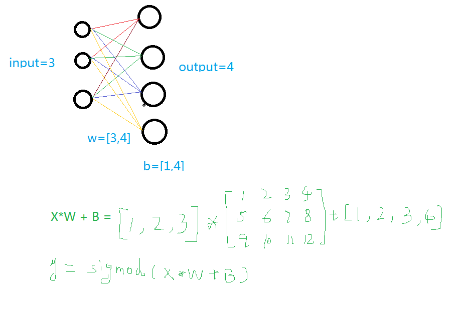
- def add_layer(inputs , in_size , out_size , activate = None):
- Weights = tf.Variable(tf.random_normal([in_size,out_size]))#随机初始化
- baises = tf.Variable(tf.zeros([1,out_size])+0.1)#可以随机但是不要初始化为0,都为固定值比随机好点
- y = tf.matmul(inputs, Weights) + baises #matmul:矩阵乘法,multipy:一般是数量的乘法
- if activate:
- y = activate(y)
- return y
2.训练一个二次函数
- import tensorflow as tf
- import numpy as np
- def add_layer(inputs , in_size , out_size , activate = None):
- Weights = tf.Variable(tf.random_normal([in_size,out_size]))#随机初始化
- baises = tf.Variable(tf.zeros([1,out_size])+0.1)#可以随机但是不要初始化为0,都为固定值比随机好点
- y = tf.matmul(inputs, Weights) + baises #matmul:矩阵乘法,multipy:一般是数量的乘法
- if activate:
- y = activate(y)
- return y
- if __name__ == '__main__':
- x_data = np.linspace(-1,1,300,dtype=np.float32)[:,np.newaxis]#创建-1,1的300个数,此时为一维矩阵,后面转化为二维矩阵===[1,2,3]-->>[[1,2,3]]
- noise = np.random.normal(0,0.05,x_data.shape).astype(np.float32)#噪声是(1,300)格式,0-0.05大小
- y_data = np.square(x_data) - 0.5 + noise #带有噪声的抛物线
- xs = tf.placeholder(tf.float32,[None,1]) #外界输入数据
- ys = tf.placeholder(tf.float32,[None,1])
- l1 = add_layer(xs,1,10,activate=tf.nn.relu)
- prediction = add_layer(l1,10,1,activate=None)
- loss = tf.reduce_mean(tf.reduce_sum(tf.square(ys - prediction),reduction_indices=[1]))#误差
- train_step = tf.train.GradientDescentOptimizer(0.1).minimize(loss)#对误差进行梯度优化,步伐为0.1
- sess = tf.Session()
- sess.run( tf.global_variables_initializer())
- for i in range(1000):
- sess.run(train_step, feed_dict={xs: x_data, ys: y_data})#训练
- if i%50 == 0:
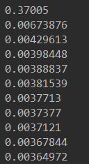
- print(sess.run(loss, feed_dict={xs: x_data, ys: y_data}))#查看误差
3.动态显示训练过程
显示的步骤程序之中部分进行说明,其它说明请看其它博客(http://www.cnblogs.com/wjy-lulu/p/7735987.html)
- import tensorflow as tf
- import numpy as np
- import matplotlib.pyplot as plt
- def add_layer(inputs , in_size , out_size , activate = None):
- Weights = tf.Variable(tf.random_normal([in_size,out_size]))#随机初始化
- baises = tf.Variable(tf.zeros([1,out_size])+0.1)#可以随机但是不要初始化为0,都为固定值比随机好点
- y = tf.matmul(inputs, Weights) + baises #matmul:矩阵乘法,multipy:一般是数量的乘法
- if activate:
- y = activate(y)
- return y
- if __name__ == '__main__':
- x_data = np.linspace(-1,1,300,dtype=np.float32)[:,np.newaxis]#创建-1,1的300个数,此时为一维矩阵,后面转化为二维矩阵===[1,2,3]-->>[[1,2,3]]
- noise = np.random.normal(0,0.05,x_data.shape).astype(np.float32)#噪声是(1,300)格式,0-0.05大小
- y_data = np.square(x_data) - 0.5 + noise #带有噪声的抛物线
- fig = plt.figure('show_data')# figure("data")指定图表名称
- ax = fig.add_subplot(111)
- ax.scatter(x_data,y_data)
- plt.ion()
- plt.show()
- xs = tf.placeholder(tf.float32,[None,1]) #外界输入数据
- ys = tf.placeholder(tf.float32,[None,1])
- l1 = add_layer(xs,1,10,activate=tf.nn.relu)
- prediction = add_layer(l1,10,1,activate=None)
- loss = tf.reduce_mean(tf.reduce_sum(tf.square(ys - prediction),reduction_indices=[1]))#误差
- train_step = tf.train.GradientDescentOptimizer(0.1).minimize(loss)#对误差进行梯度优化,步伐为0.1
- sess = tf.Session()
- sess.run( tf.global_variables_initializer())
- for i in range(1000):
- sess.run(train_step, feed_dict={xs: x_data, ys: y_data})#训练
- if i%50 == 0:
- try:
- ax.lines.remove(lines[0])
- except Exception:
- pass
- prediction_value = sess.run(prediction, feed_dict={xs: x_data})
- lines = ax.plot(x_data,prediction_value,"r",lw = 3)
- print(sess.run(loss, feed_dict={xs: x_data, ys: y_data}))#查看误差
- plt.pause(2)
- while True:
- plt.pause(0.01)
4.TensorBoard整体结构化显示
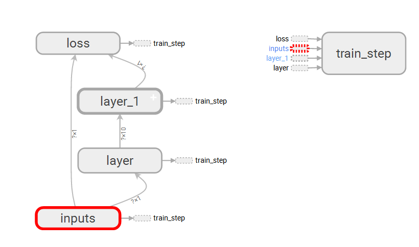
A.利用with tf.name_scope("name")创建大结构、利用函数的name="name"去创建小结构:tf.placeholder(tf.float32,[None,1],name="x_data")
B.利用writer = tf.summary.FileWriter("G:/test/",graph=sess.graph)创建一个graph文件
C.利用TessorBoard去执行这个文件
这里得注意--->>>首先到你存放文件的上一个目录--->>然后再去运行这个文件
tensorboard --logdir=test
(被屏蔽的GIF动图,具体安装操作欢迎戳“原文链接”哈!)
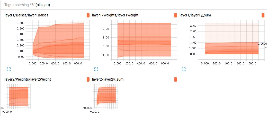
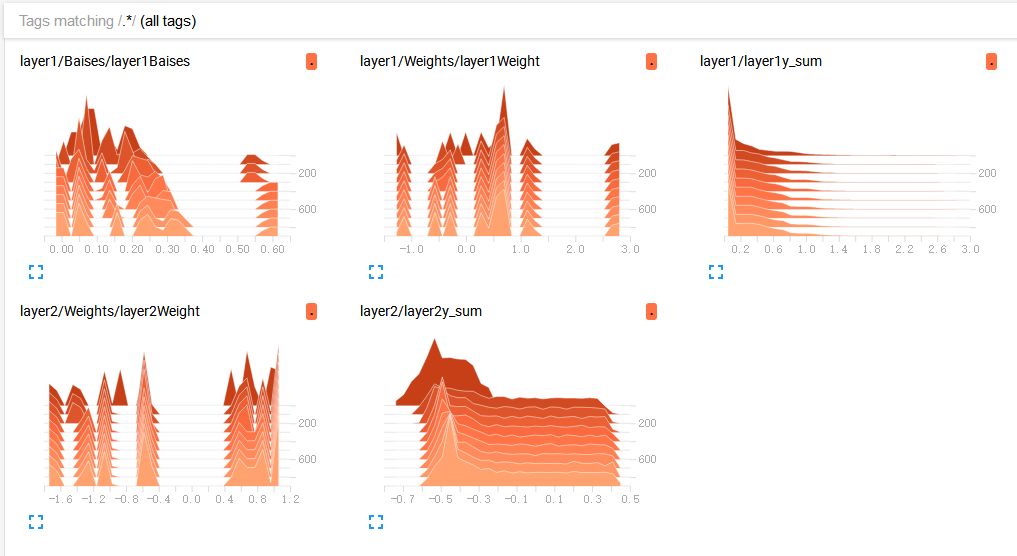
5.TensorBoard局部结构化显示
A. tf.summary.histogram(layer_name+"Weight",Weights):直方图显示
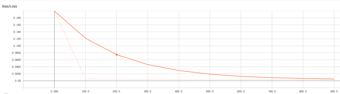
B. tf.summary.scalar("Loss",loss):折线图显示,loss的走向决定你的网络训练的好坏,至关重要一点
C.初始化与运行设定的图表
- merge = tf.summary.merge_all()#合并图表2 writer = tf.summary.FileWriter("G:/test/",graph=sess.graph)#写进文件3 result = sess.run(merge,feed_dict={xs:x_data,ys:y_data})#运行打包的图表merge4 writer.add_summary(result,i)#写入文件,并且单步长50
完整代码及显示效果:
- import tensorflow as tf
- import numpy as np
- import matplotlib.pyplot as plt
- def add_layer(inputs , in_size , out_size , n_layer = 1 , activate = None):
- layer_name = "layer" + str(n_layer)
- with tf.name_scope(layer_name):
- with tf.name_scope("Weights"):
- Weights = tf.Variable(tf.random_normal([in_size,out_size]),name="W")#随机初始化
- tf.summary.histogram(layer_name+"Weight",Weights)
- with tf.name_scope("Baises"):
- baises = tf.Variable(tf.zeros([1,out_size])+0.1,name="B")#可以随机但是不要初始化为0,都为固定值比随机好点
- tf.summary.histogram(layer_name+"Baises",baises)
- y = tf.matmul(inputs, Weights) + baises #matmul:矩阵乘法,multipy:一般是数量的乘法
- if activate:
- y = activate(y)
- tf.summary.histogram(layer_name+"y_sum",y)
- return y
- if __name__ == '__main__':
- x_data = np.linspace(-1,1,300,dtype=np.float32)[:,np.newaxis]#创建-1,1的300个数,此时为一维矩阵,后面转化为二维矩阵===[1,2,3]-->>[[1,2,3]]
- noise = np.random.normal(0,0.05,x_data.shape).astype(np.float32)#噪声是(1,300)格式,0-0.05大小
- y_data = np.square(x_data) - 0.5 + noise #带有噪声的抛物线
- fig = plt.figure('show_data')# figure("data")指定图表名称
- ax = fig.add_subplot(111)
- ax.scatter(x_data,y_data)
- plt.ion()
- plt.show()
- with tf.name_scope("inputs"):
- xs = tf.placeholder(tf.float32,[None,1],name="x_data") #外界输入数据
- ys = tf.placeholder(tf.float32,[None,1],name="y_data")
- l1 = add_layer(xs,1,10,n_layer=1,activate=tf.nn.relu)
- prediction = add_layer(l1,10,1,n_layer=2,activate=None)
- with tf.name_scope("loss"):
- loss = tf.reduce_mean(tf.reduce_sum(tf.square(ys - prediction),reduction_indices=[1]))#误差
- tf.summary.scalar("Loss",loss)
- with tf.name_scope("train_step"):
- train_step = tf.train.GradientDescentOptimizer(0.1).minimize(loss)#对误差进行梯度优化,步伐为0.1
- sess = tf.Session()
- merge = tf.summary.merge_all()#合并
- writer = tf.summary.FileWriter("G:/test/",graph=sess.graph)
- sess.run( tf.global_variables_initializer())
- for i in range(1000):
- sess.run(train_step, feed_dict={xs: x_data, ys: y_data})#训练
- if i%100 == 0:
- result = sess.run(merge,feed_dict={xs:x_data,ys:y_data})#运行打包的图表merge
- writer.add_summary(result,i)#写入文件,并且单步长50
主要参考莫凡大大:https://morvanzhou.github.io/
可视化出现问题了,参考这位大神:http://blog.csdn.net/fengying2016/article/details/54289931