利用TensorFlow和神经网络来处理文本分类问题-神经网络文本分类算法

在这篇文章中，作者讨论了六个关于创建机器学习模型来进行文本分类的主要话题。

TensorFlow 如何工作
机器学习模型是什么
神经网络是什么
神经网络怎样进行学习
如何处理数据并且把它们传输给神经网络的输入
怎样运行模型并且得到预测结果

作者也提供了可在Jupyter notebook上运行的代码。我将回顾这六个话题并且与我自己的经验相结合。

1. TensorFlow 概览

TensorFlow 是***的开源 AI 库之一。它的高计算效率，丰富的开发资源使它被企业和个人开发者广泛采用。在我看来，学习 TensorFlow 的***的方法就是使用它的官网教程(https://www.tensorflow.org/)。在这个网站上，你可以浏览「getting started」教程。

我首先将会对 TensorFlow 的基本定义和主要特征进行介绍。张量(Tensor)是一种数据结构，它可以把原始值形成任意的多维数组【1】。张量的级别就是它的维度数。这里，我建议阅读 Python 的应用编程接口 API，因为它对 TensorFlow 的初学者来说是很友好的。你可以安装 TensorFlow 并且配置环境，紧随官方网站上的指导就可以了。测试你是否成功安装 TensorFlow 的方法就是导入(import)TensorFlow 库。在 TensorFlow 中，计算图(computational graph)是核心部件。数据流程图形用来代表计算过程。在图形下，操作(Operation)代表计算单位，张量代表数据单位。为了运行代码，我们应该对阶段函数(Session function)进行初始化。这里是执行求和操作的完整代码。

#import the library 
import tensorflow as tf 
#build the graph and name as my_graph 
my_graph = tf.Graph() 
#tf.Session encapsulate the environment for my_graph 
with my_graph.as_default(): 
   x = tf.constant([1,3,6])  
   y = tf.constant([1,1,1]) 
   #add function 
   op = tf.add(x,y) 
   #run it by fetches 
   result = sess.run(fetches=op) 
   #print it 
   print(result) 
1.
2.
3.
4.
5.
6.
7.
8.
9.
10.
11.
12.
13.
14.

你可以看见在 TensorFlow 中编译是遵循一种模式的，并且很容易被记住。你将会导入库，创建恒定张量(constant tensors)并且创建图形。然后我们应该定义哪一个图将会被在 Session 中使用，并且定义操作单元。最终你可以在 Session 中使用 run() 的方法，并且评估其中参数获取的每一个张量。

2. 预测模型

预测模型可以很简单。它把机器学习算法和数据集相结合。创建一个模型的过程程如下图所示：

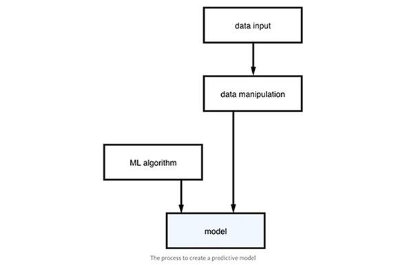
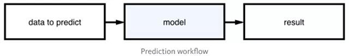
我们首先应该找到正确的数据作为输入，并且使用一些数据处理函数来处理数据。然后，这些数据就可以与机器学习算法结合来创建模型了。在你得到模型后，你可以把模型当做一个预测器并且输入需要的数据来预测，从而产生结果。整个进程如下图所示：

在本文中，输入是文本，输出结果是类别(category)。这种机器学习算法叫做监督学习，训练数据集是已标注过种类的文本。这也是分类任务，而且是应用神经网络来进行模型创建的。

3. 神经网络

神经网络的主要特征是自学(self-learning)，而不是进行明确地程序化。它的灵感来源于人类中枢神经系统。***个神经网络算法是感知机(Perceptron)。

为了理解神经网络的工作机制，作者用 TensorFlow 创建了一个神经网络结构。

(1) 神经网络结构

这里作者使用了两个隐蔽层(hidden layers)，每一个隐蔽层的职责是把输入转换成输出层可以使用的东西【1】。***个隐蔽层的节点的数量应该被定义。这些节点叫做神经元，和权值相乘。训练阶段是为了对这些值进行调节，为了产生一个正确的输出。网络也引入了偏差(bias)，这就可以让你向左或向右移动激活函数，从而让预测结果更加准确【2】。数据还会经过一个定义每个神经元最终输出的激活函数。这里，作者使用的是修正线性单元(ReLU)，可以增加非线性。这个函数被定义为：

f(x) = max(0,x)（输出是 x 或 0，无论 x 多大） 
1.

对第二个隐蔽层来说，输入就是***层，函数与***个隐蔽层相同。

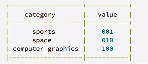
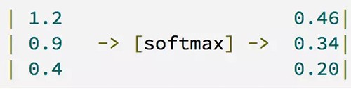
对于输出层，作者使用的是 one-hot 编码来得到结果。在 one-hot 编码中，除了其中的一位值为 1 以外，所有的位元(bits)都会得到一个 0 值。这里使用三种类别作为范例，如下图所示。

我们可以发现输出节点的数量值就是类别的数量值。如果我们想要划分不同的类别，我们可以使用 Softmax 函数来使每一个单元的输出转化成 0 到 1 间的值，并且使所有单元的总和为 1。它将会告诉我们每种类别的概率是多少。

上述过程由下列代码实现：

# Network Parameters 
n_hidden_1 = 10        # 1st layer number of features 
n_hidden_2 = 5         # 2nd layer number of features 
n_input = total_words  # Words in vocab 
n_classes = 3          # Categories: graphics, space and baseball 
1.
2.
3.
4.
5.

def multilayer_perceptron(input_tensor, weights, biases): 
    layer_1_multiplication = tf.matmul(input_tensor, weights['h1']) 
    layer_1_addition = tf.add(layer_1_multiplication, biases['b1']) 
    layer_1_activation = tf.nn.relu(layer_1_addition) 
1.
2.
3.
4.

# Hidden layer with RELU activation 
    layer_2_multiplication = tf.matmul(layer_1_activation, weights['h2']) 
    layer_2_addition = tf.add(layer_2_multiplication, biases['b2']) 
    layer_2_activation = tf.nn.relu(layer_2_addition) 
1.
2.
3.
4.

# Output layer with linear activation 
    out_layer_multiplication = tf.matmul(layer_2_activation, weights['out']) 
    out_layer_addition = out_layer_multiplication + biases['out'] 
1.
2.
3.

return out_layer_addition 
1.

在这里，它调用了 matmul()函数来实现矩阵之间的乘法函数，并调用 add()函数将偏差添加到函数中。

4. 神经网络是如何训练的

我们可以看到其中要点是构建一个合理的结构，并优化网络权重的预测。接下来我们需要训练 TensorFlow 中的神经网络。在 TensorFlow 中，我们使用 Variable 来存储权重和偏差。在这里，我们应该将输出值与预期值进行比较，并指导函数获得最小损失结果。有很多方法来计算损失函数，由于它是一个分类任务，所以我们应该使用交叉熵误差。此前 D. McCaffrey[3] 分析并认为交叉熵可以避免训练停滞不前。我们在这里通过调用函数 tf.nn.softmax_cross_entropy_with_logits() 来使用交叉熵误差，我们还将通过调用 function: tf.reduced_mean() 来计算误差。

# Construct model 
prediction = multilayer_perceptron(input_tensor, weights, biases) 
1.
2.

# Define loss 
entropy_loss = tf.nn.softmax_cross_entropy_with_logits(logits=prediction, labels=output_tensor) 
loss = tf.reduce_mean(entropy_loss) 
1.
2.
3.

我们应该找到***值来使输出误差最小化。这里我们使用随机梯度下降(SGD)的方法：

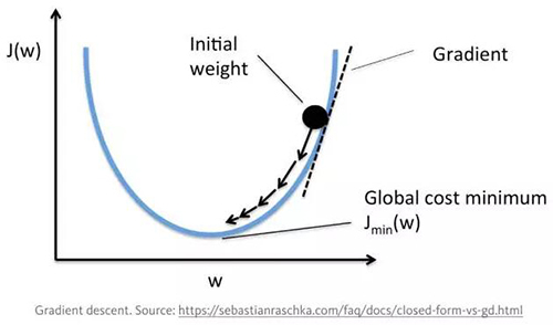
通过多次迭代，我们将会得到接近于全局最小损失的权值。学习速率不应该太大。自适应瞬间评估函数(Adaptive Moment Estimation function)经常用于计算梯度下降。在这个优化算法中，对梯度和梯度的二阶矩量进行平滑处理【4】。

代码如下所示，在其它项目中，学习速率可以是动态的，从而使训练过程更加迅速。

learning_rate = 0.001 
# Construct model 
prediction = multilayer_perceptron(input_tensor, weights, biases) 
1.
2.
3.

# Define loss 
entropy_loss = tf.nn.softmax_cross_entropy_with_logits(logits=prediction, labels=output_tensor) 
loss = tf.reduce_mean(entropy_loss) 
1.
2.
3.

optimizer = tf.train.AdamOptimizer(learning_ratelearning_rate=learning_rate).minimize(loss) 
1.

5. 数据操作

这一部分对于分类成功也很重要。机器学习的开发者们需要更加在意数据，这会为你节省大量时间，并让结果更加准确，因为这可以让你无需从头开始更改配置。在这里，笔者需要指出两个重点。首先，为每个单词创建一个索引;然后为每个文本创建一个矩阵，如果单词在文本中，则值为 1，否则为 0。以下代码可以帮助你理解这个过程：

import numpy as np    #numpy is a package for scientific computing 
from collections import Counter 
1.
2.

vocab = Counter() 
text = "Hi from Brazil" 
#Get all words 
for word in text.split(' '): 
    vocab[word]+=1 
         
#Convert words to indexes 
def get_word_2_index(vocab): 
    word2index = {} 
    for i,word in enumerate(vocab): 
        word2index[word] = i 
         
    return word2index 
#Now we have an index 
word2index = get_word_2_index(vocab) 
total_words = len(vocab) 
#This is how we create a numpy array (our matrix) 
matrix = np.zeros((total_words),dtype=float) 
#Now we fill the values 
for word in text.split(): 
    matrix[word2index[word]] += 1 
print(matrix) 
>>> [ 1.  1.  1.] 
1.
2.
3.
4.
5.
6.
7.
8.
9.
10.
11.
12.
13.
14.
15.
16.
17.
18.
19.
20.
21.
22.
23.

Python 中的 Counter() 是一个哈希表。当输入是「Hi from Brazil」时，矩阵是 [1 ,1, 1]。如果输入不同，比如「Hi」，矩阵会得到不同的结果：

matrix = np.zeros((total_words),dtype=float) 
text = "Hi" 
for word in text.split(): 
    matrix[word2index[word.lower()]] += 1 
print(matrix) 
>>> [ 1.  0.  0.] 
1.
2.
3.
4.
5.
6.

6. 运行模型，获得结果

在这一部分里，我们将使用 20 Newsgroups 作为数据集。它包含有关 20 种话题的 18,000 篇文章。我们使用 scilit-learn 库加载数据。在这里作者使用了 3 个类别：comp.graphics、sci.space 和 rec.sport.baseball。它有两个子集，一个用于训练，一个用于测试。下面是加载数据集的方式：

from sklearn.datasets import fetch_20newsgroups 
categories = ["comp.graphics","sci.space","rec.sport.baseb 
1.
2.

newsgroups_train = fetch_20newsgroups(subset='train', categoriescategories=categories) 
newsgroups_test = fetch_20newsgroups(subset='test', categoriescategories=categories) 
1.
2.

它遵循通用的模式，非常易于开发者使用。

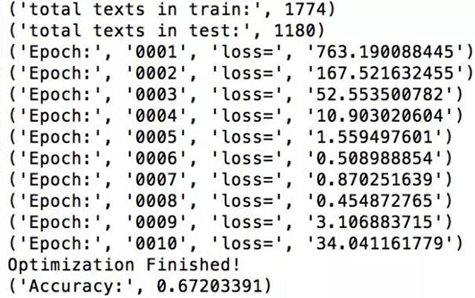
在实验中，epoch 设定为 10，这意味着会有 10 次正+反向遍历整个数据集。在 TensorFlow 中，占位符的作用是用作 Feed 的目标，用于传递每个运行步骤的数据。

n_input = total_words # Words in vocab 
n_classes = 3         # Categories: graphics, sci.space and baseball 
1.
2.

input_tensor = tf.placeholder(tf.float32,[None, n_input],name="input") 
output_tensor = tf.placeholder(tf.float32,[None, n_classes],name="output") 
1.
2.

我们应该分批训练数据，因为在测试模型时，我们会用更大的批次来输入 dict。调用 get_batches() 函数来获取具有批处理尺寸的文本数。接下来，我们就可以运行模型了。

training_epochs = 10 
# Launch the graph 
with tf.Session() as sess: 
    sess.run(init) #inits the variables (normal distribution, reme 
1.
2.
3.
4.

# Training cycle 
   for epoch in range(training_epochs): 
       avg_cost = 0. 
       total_batch = int(len(newsgroups_train.data)/batch_size) 
       # Loop over all batches 
       for i in range(total_batch): 
           batch_x,batch_y = get_batch(newsgroups_train,i,batch_size) 
           # Run optimization op (backprop) and cost op (to get loss value) 
           c,_ = sess.run([loss,optimizer], feed_dict={input_tensor: batch_x, output_tensor:batch_y}) 
1.
2.
3.
4.
5.
6.
7.
8.
9.

在这里我们需要构建测试模型，并计算它的准确性。

# Test model 
    index_prediction = tf.argmax(prediction, 1) 
    index_correct = tf.argmax(output_tensor, 1) 
    correct_prediction = tf.equal(index_prediction, index_correct) 
1.
2.
3.
4.

# Calculate accuracy 
   accuracy = tf.reduce_mean(tf.cast(correct_prediction, "float")) 
   total_test_data = len(newsgroups_test.target) 
   batch_x_test,batch_y_test = get_batch(newsgroups_test,0,total_test_data) 
   print("Accuracy:", accuracy.eval({input_tensor: batch_x_test, output_tensor: batch_y_test})) 
1.
2.
3.
4.
5.

然后我们就可以得到结果：

结论

本文介绍了如何使用神经网络和 TensorFlow 来处理文本分类任务。它介绍了与实验有关的基础信息，然而，在我自己运行的时候，效果就没有作者那么好了。我们或许可以在这个架构的基础上改进一番，在隐藏层中使用 dropout 肯定会提高准确性。

在运行代码前，请确认你已安装了***版本的 TensorFlow。有些时候你可能会无法导入 twenty_newsgroups 数据集。当这种情况发生时，请使用以下代码来解决问题。

# if you didn't download the twenty_newsgroups datasets, it will run with error 
# this logging can help to solve the error 
import logging 
logging.basicConfig() 
1.
2.
3.
4.

以下是完整代码：

import pandas as pd 
import numpy as np 
import tensorflow as tf 
from collections import Counter 
from sklearn.datasets import fetch_20newsgroups 
# if you didn't download the twenty_newsgroups datasets, it will run with error 
# this logging can help to solve the error 
import logging 
logging.basicConfig() 
 
categories = ["comp.graphics","sci.space","rec.sport.baseball"] 
newsgroups_train = fetch_20newsgroups(subset='train', categoriescategories=categories) 
newsgroups_test = fetch_20newsgroups(subset='test', categoriescategories=categories) 
 
print('total texts in train:',len(newsgroups_train.data)) 
print('total texts in test:',len(newsgroups_test.data)) 
 
vocab = Counter() 
for text in newsgroups_train.data: 
   for word in text.split(' '): 
       vocab[word.lower()]+=1 
        
for text in newsgroups_test.data: 
   for word in text.split(' '): 
       vocab[word.lower()]+=1 
 
 
total_words = len(vocab) 
def get_word_2_index(vocab): 
   word2index = {} 
   for i,word in enumerate(vocab): 
       word2index[word.lower()] = i 
        
   return word2index 
 
word2index = get_word_2_index(vocab) 
 
def get_batch(df,i,batch_size): 
   batches = [] 
   results = [] 
   texts = df.data[i*batch_size:i*batch_size+batch_size] 
   categories = df.target[i*batch_size:i*batch_size+batch_size] 
   for text in texts: 
       layer = np.zeros(total_words,dtype=float) 
       for word in text.split(' '): 
           layer[word2index[word.lower()]] += 1 
            
       batches.append(layer) 
        
   for category in categories: 
       y = np.zeros((3),dtype=float) 
       if category == 0: 
           y[0] = 1. 
       elif category == 1: 
           y[1] = 1. 
       else: 
           y[2] = 1. 
       results.append(y) 
            
     
   return np.array(batches),np.array(results) 
 
# Parameters 
learning_rate = 0.01 
training_epochs = 10 
batch_size = 150 
display_step = 1 
 
# Network Parameters 
n_hidden_1 = 100      # 1st layer number of features 
n_hidden_2 = 100       # 2nd layer number of features 
n_input = total_words # Words in vocab 
n_classes = 3         # Categories: graphics, sci.space and baseball 
 
input_tensor = tf.placeholder(tf.float32,[None, n_input],name="input") 
output_tensor = tf.placeholder(tf.float32,[None, n_classes],name="output")  
 
def multilayer_perceptron(input_tensor, weights, biases): 
   layer_1_multiplication = tf.matmul(input_tensor, weights['h1']) 
   layer_1_addition = tf.add(layer_1_multiplication, biases['b1']) 
   layer_1 = tf.nn.relu(layer_1_addition) 
    
   # Hidden layer with RELU activation 
   layer_2_multiplication = tf.matmul(layer_1, weights['h2']) 
   layer_2_addition = tf.add(layer_2_multiplication, biases['b2']) 
   layer_2 = tf.nn.relu(layer_2_addition) 
    
   # Output layer  
   out_layer_multiplication = tf.matmul(layer_2, weights['out']) 
   out_layer_addition = out_layer_multiplication + biases['out'] 
    
   return out_layer_addition 
 
# Store layers weight & bias 
weights = { 
   'h1': tf.Variable(tf.random_normal([n_input, n_hidden_1])), 
   'h2': tf.Variable(tf.random_normal([n_hidden_1, n_hidden_2])), 
   'out': tf.Variable(tf.random_normal([n_hidden_2, n_classes])) 
} 
biases = { 
   'b1': tf.Variable(tf.random_normal([n_hidden_1])), 
   'b2': tf.Variable(tf.random_normal([n_hidden_2])), 
   'out': tf.Variable(tf.random_normal([n_classes])) 
} 
 
# Construct model 
prediction = multilayer_perceptron(input_tensor, weights, biases) 
 
# Define loss and optimizer 
loss = tf.reduce_mean(tf.nn.softmax_cross_entropy_with_logits(logits=prediction, labels=output_tensor)) 
optimizer = tf.train.AdamOptimizer(learning_ratelearning_rate=learning_rate).minimize(loss) 
 
# Initializing the variables 
init = tf.initialize_all_variables() 
 
# Launch the graph 
with tf.Session() as sess: 
   sess.run(init) 
 
   # Training cycle 
   for epoch in range(training_epochs): 
       avg_cost = 0. 
       total_batch = int(len(newsgroups_train.data)/batch_size) 
       # Loop over all batches 
       for i in range(total_batch): 
           batch_x,batch_y = get_batch(newsgroups_train,i,batch_size) 
           # Run optimization op (backprop) and cost op (to get loss value) 
           c,_ = sess.run([loss,optimizer], feed_dict={input_tensor: batch_x,output_tensor:batch_y}) 
           # Compute average loss 
           avg_cost += c / total_batch 
       # Display logs per epoch step 
       if epoch % display_step == 0: 
           print("Epoch:", '%04d' % (epoch+1), "loss=", \ 
               "{:.9f}".format(avg_cost)) 
   print("Optimization Finished!") 
 
   # Test model 
   correct_prediction = tf.equal(tf.argmax(prediction, 1), tf.argmax(output_tensor, 1)) 
   # Calculate accuracy 
   accuracy = tf.reduce_mean(tf.cast(correct_prediction, "float")) 
   total_test_data = len(newsgroups_test.target) 
   batch_x_test,batch_y_test = get_batch(newsgroups_test,0,total_test_data) 
   print("Accuracy:", accuracy.eval({input_tensor: batch_x_test, output_tensor: batch_y_test})) 
1.
2.
3.
4.
5.
6.
7.
8.
9.
10.
11.
12.
13.
14.
15.
16.
17.
18.
19.
20.
21.
22.
23.
24.
25.
26.
27.
28.
29.
30.
31.
32.
33.
34.
35.
36.
37.
38.
39.
40.
41.
42.
43.
44.
45.
46.
47.
48.
49.
50.
51.
52.
53.
54.
55.
56.
57.
58.
59.
60.
61.
62.
63.
64.
65.
66.
67.
68.
69.
70.
71.
72.
73.
74.
75.
76.
77.
78.
79.
80.
81.
82.
83.
84.
85.
86.
87.
88.
89.
90.
91.
92.
93.
94.
95.
96.
97.
98.
99.
100.
101.
102.
103.
104.
105.
106.
107.
108.
109.
110.
111.
112.
113.
114.
115.
116.
117.
118.
119.
120.
121.
122.
123.
124.
125.
126.
127.
128.
129.
130.
131.
132.
133.
134.
135.
136.
137.
138.
139.
140.
141.
142.
143.

【本文是51CTO专栏机构“机器之心”的原创文章，微信公众号“机器之心( id: almosthuman2014)”】

戳这里，看该作者更多好文